Download
1 / 44
440 likes | 735 Views
Atmospheric Tracers and the Great Lakes. Ankur R Desai University of Wisconsin. Questions. Can we “see” Lake Superior in the atmosphere? Lake effect. Lake Effect. Source: Wikimedia Commons. Lake Effect. Source: S.Spak, UW SAGE. Questions. Can we “see” Lake Superior in the atmosphere?

E N D
Atmospheric Tracers and the Great Lakes Ankur R Desai University of Wisconsin
Questions • Can we “see” Lake Superior in the atmosphere? • Lake effect
Lake Effect • Source: Wikimedia Commons
Lake Effect • Source: S.Spak, UW SAGE
Questions • Can we “see” Lake Superior in the atmosphere? • Lake effect • Carbon effect? • If so, can we constrain air-lake exchange by atmospheric observations? • If that, can we compare terrestrial and aquatic regional fluxes?
Carbon Effect? • Is the NOAA/UW/PSU WLEF tall tower greenhouse gas observatory adequate for sampling Lake Superior air?
First • A little bit about atmospheric tracers and inversions…
Classic Inversion • Source: S. Denning, CSU
Regional Sources/Sinks • Global cooperative sampling network not sufficient to detail processes at sub-seasonal, sub-continental, and sub-biome scale • Weekly/monthly sampling • Low spatial density • Poorly constrained inversion
Regional Sources/Sinks • Global cooperative sampling network not sufficient to detail processes at sub-seasonal, sub-continental, and sub-biome scale • Weekly/monthly sampling • Low spatial density • Poorly constrained inversion
Where We See • Surface footprint influence function for tracer concentrations can be computed with LaGrangian ensemble back trajectories • transport model wind fields, mixing depths (WRF) • particle model (STILT)
Where We See • Source: A. Andrews, NOAA ESRL
Regional Sources/Sinks • Global cooperative sampling network not sufficient to detail processes at sub-seasonal, sub-continental, and sub-biome scale • Weekly/monthly sampling • Low spatial density • Poorly constrained inversion
Regional Sources/Sinks • Global cooperative sampling network not sufficient to detail processes at sub-seasonal, sub-continental, and sub-biome scale • Weekly/monthly sampling • Low spatial density • Poorly constrained inversion
Terrestrial Flux • Annual NEE (gC m-2 yr-1) -160 (-60 – -320) • Buffam et al (submitted) -200
Problems With Regional Inversions • It is still an under-constrained problem! • Assumptions about surface forcing can skew results • Great Lakes are usually ignored • Sensitive to assumptions about “inflow” fluxes • Sensitive to error covariance structure in Bayesian optimization • Transport models have more error at higher resolution • Great Lakes have complex meteorology
Simpler Techniques • Boundary Layer Budgeting • Compare [CO2] of lake and non-lake trajectory air • WRF-STILT nested grid tracer transport model • Estimate boundary layer depth and advection timescale to yield flux • Equilibrium Boundary Layer • Compare [CO2] of free troposphere and boundary layer air averaged over synoptic cycles • Estimate subsidence rate to yield flux
There Is a Lake Signal • Source: N. Urban (MTU)
We Might See It at WLEF • Source: M. Uliasz, CSU
EBL method (Helliker et al, 2004) Mixed layer Free troposphere Surface flux
Onward • Trajectory analysis and simple budgets – see next talk by Victoria Vasys • Attempting regional flux inversions with lakes explicitly considered – in progress (A. Schuh, CSU) • Direct eddy flux measurements over the lake – in progress (P. Blanken, CU; N. Urban, MTU)
Trout Lake NEE (preliminary) • Source: M. Balliett, UW
Thanks! • CyCLeS project: G. Mckinley, N. Urban, C. Wu, V. Bennington, N. Atilla, C. Mouw, and others, NSF • NSF REU: Victoria Vasys • WLEF: A. Andrews, NOAA ESRL, R. Strand, WI ECB; J. Thom, UW; R. Teclaw, D. Baumann, USFS NRS • WRF-STILT: A. Michalak, D. Huntzinger, S. Gourdji, U. Michigan; J. Eluszkiewicz, AER • Regional Inversions: M. Uliasz, S. Denning, A. Schuh, CSU • EBL: B. Helliker, U. Penn • Eddy flux: P. Blanken, CU