Download

1 / 42
550 likes | 1.45k Views
Experimental Fluid Dynamics and Uncertainty Assessment Methodology. S. Ghosh, M. Muste, F. Stern. Table of. Definition & purpose EFD philosophy EFD Process Types of measurements & instrumentation Measurement systems Uncertainty analysis 57:020 Laboratories. Experimental Fluid Dynamics.

E N D
Experimental Fluid Dynamics and Uncertainty Assessment Methodology S. Ghosh, M. Muste, F. Stern
Table of • Definition & purpose • EFD philosophy • EFD Process • Types of measurements & instrumentation • Measurement systems • Uncertainty analysis • 57:020 Laboratories
Experimental Fluid Dynamics Definition: Experimental Fluid Dynamics: Use of experimental methodology and procedures for solving fluids engineering systems, including full and model scales, large and table top facilities, measurement systems (instrumentation, data acquisition and data reduction), dimensional analysis and similarity and uncertainty analysis. Purpose: • Science & Technology: understand and investigate a phenomenon/process, substantiate and validate a theory (hypothesis) • Research & Development: document a process/system, provide benchmark data (standard procedures, validations), calibrate instruments, equipment, and facilities • Industry: design optimization and analysis, provide data for direct use, product liability, and acceptance • Teaching: Instruction/demonstration A pretty experiment is in itself often more valuable than twenty formulae extracted from our minds." - Albert Einstein
EFD Philosophy • Decisions on conducting experiments are governed by the ability of the expected test outcome to achievethe experimentobjectives within allowable uncertainties. • Integration of UA into all test phases should be a key part of entire experimental program • test design • determination of error sources • estimation of uncertainty • documentation of the results
EFD Process • EFD labs provide “hands on” experience with modern measurement systems, understanding and implementation of EFD in practical application and focus on “EFD process”:
Measurement systems • Instrumentation (sensors, probes) • Data acquisition • Serial port devices • Analog to Digital (A/D) converters • Signal conditioners/filters • Plug-in data acquisition boards • Desktop PC’s • DA software - Labview • Data analysis and data reduction • Data reduction equations • Curve fitting techniques • Statistical techniques • Spectral analysis (Fast Fourier Transform) • Proper orthogonal decomposition • Data visualizations
Manometers • Principle of operation:Manometers are devices in which columns of suitable liquid are used to measure the difference in pressure between two points, or between a certain point and the atmosphere (patm). • Applying fundamental equations of hydrostatics the pressure difference, P, between the two liquid columns can be calculated. • Manometers are frequently used to measure pressure differences sensed by Pitot tubes to determine velocities in various flows. • Types of manometers: simple, differential (U-tube), inclined tube, high precision (Rouse manometer). U-tube manometer
Inclined-tube manometer Inclined tube manometer • Used for accurate measurement of small pressure differences • The density of manometric fluid is not equal to that of the working fluid (e.g. working fluid is gas) • is small to magnify the meniscus movement compared with a vertical tube • Angles less than 5 are not usually recommended.
Pressure transducers A pressure transducer converts the pressure sensed by the instrument probe into mechanical or electrical signals Pressure transducer Elastic elements used to convert pressure within transducers Transducer read out
Pressure transducers Schematic of a membrane-based pressure transducer • A a diaphragm separates the high and low incoming pressures. • The diaphragm deflects under the pressure differencethus changing the capacitance(C) of the circuit, which eventually changes the voltage output(E). • The voltages are converted through calibrations to pressure units. • Pressure transducers are used with pressure taps, pitot tubes, pulmonary functions, HVAC, mechanical pressures, etc.
Pressure taps • Static(Pstat) and stagnation(Pstag) pressures • Pressure caused only by molecular collisions is known as static pressure. • The pressure tap is a small opening in the wall of a a duct (Fig a.) • Pressure tap connected to any pressure measuring device indicates the static pressure. (note: there is no component of velocity along the tap axis). • The stagnation pressure at a point in a fluid flow is the pressure that could result if the fluid was brought to rest isentropically (i.e., the entire kinetic energy of the fluid is utilized to increase its pressure only). Single and multi pressure taps
Bernoulli’s Equation 2 For an incompressible flow with no heat or work exchange, the mechanical energy equation can be written as 1 Z2 Flow direction Z1 Reference level • Assumptions: • energy is conserved along a streamline • incompressible flow • no work or heat interaction
Pitot tube • Principle of pitot tube operation • The tubes sensing static and stagnation pressures are usually combined into one instrument known as pitot static tube. • Pressure taps sensing static pressure (also the reference pressure for this measurement) are placed radially on the probe stem and then combined into one tube leading to the differential manometer (pstat). • The pressure tap located at the probe tip senses the stagnation pressure (p0). • Use of the two measured pressures in the Bernoulli equation allows to determine one component of the flow velocity at the probe location. • Special arrangements of the pressure taps (Three-hole, Five-hole, seven-hole Pitot) in conjunction with special calibrations are used two measure all velocity components. • It is difficult to measure stagnation pressure in real, due to friction. The measured stagnation pressure is always less than the actual one. This is taken care of by an empirical factor C. P0 = stagnation pressure Pstat = static pressure
Venturi meter • Principle of venturi meter operation • The venturi meter consists of two conical pipes connected as shown in the figure. The minimum cross section diameter is called throat. The angles of the conical pipes are established to limit the energy losses due to flow separation. • The flow obstruction produced by the venturi meter produces a local loss that is proportional to the flow discharge. • Pressure taps are located upstream and downstream of the venturi meter, immediately outside the variable diameter areas, to measure the losses produced through the meter. • Flow rate measurements are obtained using Bernoulli equation and the continuity equation (see below the derivation). An experimental coefficient is used to account for the losses occurring in the meter (Va and Vb are the upstream and downstream velocities and r is the density. (Aa and Ab are the cross sectional areas). Volumetric flow rate
Hotwire • Single hot-wire probe • Platinum plated Tungsten • 5 m diameter, 1.2 mm length • Constant temperature anemometer • Used for mean and instantaneous (fluctuating) velocity measurements • Principle of operation: Sensor resistance is changed by the flow over the probe and the cooling taking place is related through calibration to the velocity of the incoming flow. • The tool is very reliable for the measurement of velocity fluctuations due to its high sampling frequency and small size of the probe. • Cross-wire (X) probe • Two sensors perpendicular to each other • Measures within 45
Load cell Principle Principle of Load cell operation • Load cells measure forces and moments by sensing the deformation of elastic elements such as springs. • Usually it comprises of two parts • the spring: deforms under the load (usually made of steel) • sensing element: measures the deformation (usually a strain gauge glued to the deforming element). • Load cell measurement accuracy is limited by hysteresis and creep, that can be minimized by using high-grade steel and labor intensive fabrication.
Particle Image Velocimetry [PIV] • PIV setup • Images of the flow field are captured with camera(s). • 1 camera is used for 2-dimesional flow field measurement • 2 cameras are used for stereoscopic 2-dimesional measurement, whereby a third dimension can be extracted → 3-dimensional • 3 or more cameras are used for 3-dimensional measurement • Illumination comes from laser(s), LED’s, or other lights sources • Fluid is saturated with small and neutrally buoyant particles
Particle Image Velocimetry • Principle of PIV operation • Particles in flow scatter laser(s) light • Two images, per camera, are taken within a small time of one another Δt. • Both images are divided into identical smaller sections, called interrogation windows • Patterns of particles within an interrogation window are traced • Image pixels are calibrated to a known distance • Number of pixels between a particle and the same particle Δt later == a distance • →process called cross correlation • Velocity = direction × (distance a particle travels/ Δt)
Particle Image Velocimetry • ←PIV Image #1 and #2 • Advantages of PIV • Entire velocity field can be calculated • Capability of measuring flows in 3-D space • Generally, the equipment is nonintrusive to flow • High degree of accuracy • Disadvantages of PIV • Requires proper selection of particles • Size of flow structures are limited by resolution of image • Costly • Cross correlated images provide a velocity field
Data acquisition outline • General scheme of a data acquisition hardware (one channel): • Current trends: multi-channel (simultaneous sampling), microprocessor- controlled • Special considerations: • Correlate sampling type, sampling frequency (Nyquist criterion), and sampling time with the dynamic content of the signal andthe flow nature (laminar or turbulent) • Correlate the resolution for the A/D converters with the magnitude of the signal • Identify sources of errors for each step of signal conversion
Data acquisition components • Signal conditioning • Analog multiplexers • Converters • Clock • Master controller • Digital input/output device • Input/output buffer • Output devices
DA components • Signal conditioning: Output signal from transducers are conditioned prior to sampling and digital conversion. • Analog multiplexer: Is a multiple port switch that permits multiple analog inputs to be connected to a common output. • Converters: DAS uses an analog to digital converter to sample and convert the magnitude of the analog signal into binary numbers. • Clock: Clock provides master timing for the DAS process by providing a precise stream of pulses to the various system components. • Master controller: It provides the start and stop sequences for data acquisition to control actual flow into and out of the system. • I/O device: Some transducers and measuring devices output a digital signal directly which, enables bypassing the A/D converter of the DAS. • I/O buffer: This is a digital random access memory (RAM) where the data is stored before sending it to some other storage device. • Output devices: Permanent storage or display devices (zip disk, hard disk, printer, etc.)
Signal types • Signal classification • Analog • A signal that is continuous in time • Discrete • Contains information about the signal only at discrete points in time • Assumptions are necessary about the behavior of the variable during times when it is not sampled • Sampling rate should be high so that the signal is assumed constant between the samples • Digital • Useful when data acquisition and processing are performed using a computer • Digital signal exists at discrete values in time • Magnitude of digital signal is determined by Quantization • Quantization assigns a single number to represent a range of magnitude of a continuous signal. analog discrete digital
Preprocessing analog signals Preprocessing deals with conditioning signals or optimizing signal levels to obtain desired accuracies. • Filtering : eliminate aliasing, noise removal (filtering) • Low pass filter • High pass filter • Band pass filter • Notch filter • Offset : offset voltage value subtracted from actual signal • Offset helps in assessing the intensity of fluctuation of a signal • Amplification : signal level amplified to optimally suit the hardware it is fed into • Gain helps to amplify the signal • Generally the values are amplified to take full advantage of the range of A/D converter.
Aliasing • Concept of sampling frequency : • Digitization (conversion of analog to digital signal expressed in the binary system) of analog signals is performed at equally spaced time intervals, t. • Of great importance is to determine the appropriate value of t (sampling data rate). • Accurate sampling of a fluctuating signal needs to be made with at least twice the maximum frequency in the flow (Nyquist criterion). Otherwise, aliasing occurs (confusion between low and high frequency signal components). • To eliminate aliasing, all the information in original data is removed above the Nyquist frequency (fA = 1/(2t)). Removal is achieved by using low-pass filtering that removes frequencies above fA before the data passes through the A/D conversion. Effect of sampling rate
Filtering band pass filter • Low pass filters • Permits frequencies below f • Eliminates highfrequency noise • Prevents aliasing associated with sampling process High pass filters • Permits frequencies above f • Used for suppressing contribution from certain frequency ranges Band pass filters • Permits frequencies between f1 and f2 • To get finer details in the range of interest
Data acquisition hardware Adapter cable 8 port smart switch RS232 PCI serial card 8 – channel analog input module Computerized automated data acquisition system
Data Acquisition software • Introduction to Labview • Labview is a programming software used for data acquisition, instrument control, measurement analysis, etc. • Graphical programming language that uses icons • instead of text. • Labview allows to build user interfaces with a set of tools and objects. • The user interface is called the front panel and a block diagram controls the front panel. • The program is written on the block diagram and the front panel is used to control and run the program. Labview literature
Labview - Opening a new program Labview demo
Running a Labview program Block diagram Front panel
Uncertainty Analysis • Uncertainty analysis (UA): rigorous methodology for uncertainty assessment using statistical and engineering concepts • ASME and AIAA standards (e.g., ASME, 1998; AIAA, 1995) are the most recent updates of UA methodologies, which are internationally recognized
Uncertainty Analysis Definitions • Accuracy: closeness of agreement between measured and true value • Error: difference between measured and true value • Uncertainties (U): estimate of errors in measurements of individual variables Xi (Uxi) or results (Ur) obtained by combining Uxi • Estimates of U made at 95% confidence level
Uncertainty Analysis Block diagram showing elemental error sources, individual measurement systems measurement of individual variables, data reduction equations, and experimental results
Lab Schedule and Report Instructions • Lab Schedule: See the class website: http://css.engineering.uiowa.edu/~fluids/fluids.htm • Lab report instructions See the class website: http://css.engineering.uiowa.edu/~fluids/documents/ instructions_for_lab_report.pdf