Download
1 / 13

E N D
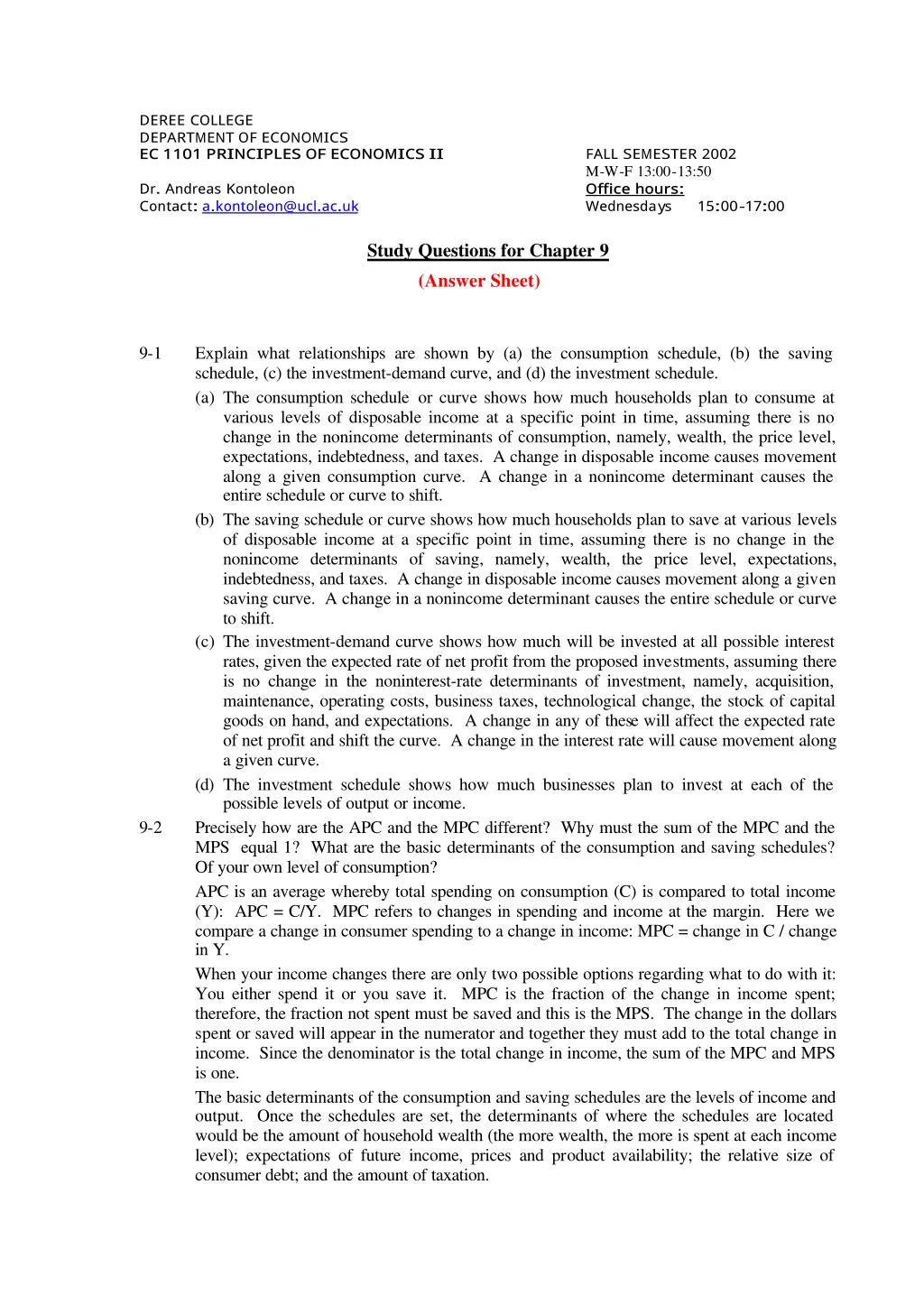
DEREE COLLEGE DEPARTMENT OF ECONOMICS EC 1101 PRINCIPLES OF ECONOMICS II FALL SEMESTER 2002 M-W-F 13:00-13:50 Office hours: Wednesdays Dr. Andreas Kontoleon Contact: a.kontoleon@ucl.ac.uk 15:00-17:00 Study Questions for Chapter 9 (Answer Sheet) 9-1 Explain what relationships are shown by (a) the consumption schedule, (b) the saving schedule, (c) the investment-demand curve, and (d) the investment schedule. (a) The consumption schedule or curve shows how much households plan to consume at various levels of disposable income at a specific point in time, assuming there is no change in the nonincome determinants of consumption, namely, wealth, the price level, expectations, indebtedness, and taxes. A change in disposable income causes movement along a given consumption curve. A change in a nonincome determinant causes the entire schedule or curve to shift. (b) The saving schedule or curve shows how much households plan to save at various levels of disposable income at a specific point in time, assuming there is no change in the nonincome determinants of saving, namely, wealth, the price level, expectations, indebtedness, and taxes. A change in disposable income causes movement along a given saving curve. A change in a nonincome determinant causes the entire schedule or curve to shift. (c) The investment-demand curve shows how much will be invested at all possible interest rates, given the expected rate of net profit from the proposed investments, assuming there is no change in the noninterest-rate determinants of investment, namely, acquisition, maintenance, operating costs, business taxes, technological change, the stock of capital goods on hand, and expectations. A change in any of these will affect the expected rate of net profit and shift the curve. A change in the interest rate will cause movement along a given curve. (d) The investment schedule shows how much businesses plan to invest at each of the possible levels of output or income. Precisely how are the APC and the MPC different? Why must the sum of the MPC and the MPS equal 1? What are the basic determinants of the consumption and saving schedules? Of your own level of consumption? APC is an average whereby total spending on consumption (C) is compared to total income (Y): APC = C/Y. MPC refers to changes in spending and income at the margin. Here we compare a change in consumer spending to a change in income: MPC = change in C / change in Y. When your income changes there are only two possible options regarding what to do with it: You either spend it or you save it. MPC is the fraction of the change in income spent; therefore, the fraction not spent must be saved and this is the MPS. The change in the dollars spent or saved will appear in the numerator and together they must add to the total change in income. Since the denominator is the total change in income, the sum of the MPC and MPS is one. The basic determinants of the consumption and saving schedules are the levels of income and output. Once the schedules are set, the determinants of where the schedules are located would be the amount of household wealth (the more wealth, the more is spent at each income level); expectations of future income, prices and product availability; the relative size of consumer debt; and the amount of taxation. 9-2
Chances are that most of us would answer that our income is the basic determinant of our levels of spending and saving, but a few may have low incomes, but with large family wealth that determines the level of spending. Likewise, other factors may enter into the pattern, as listed in the preceding paragraph. Answers will vary depending on the student’s situation. Explain how each of the following will affect the consumption and saving schedules or the investment schedule: a. A large increase in the value of real estate, including private houses. b. The threat of limited, non-nuclear war, leading the public to expect future shortages of consumer durables. c. A decline in the real interest rate. d. A sharp, sustained decline in stock prices. e. An increase in the rate of population growth. f. The development of a cheaper method of manufacturing computer chips. g. A sizable increase in the retirement age for collecting social security benefits. h. The expectation that mild inflation will persist in the next decade. i. An increase in the Federal personal income tax. (a) If this simply means households have become more wealthy, then consumption will increase at each income level. The consumption schedule should shift upward and the saving schedule shift leftward. The investment schedule may shift rightward if owners of existing homes sell them and invest in construction of new homes more than previously. (b) This threat will lead people to stock up; the consumption schedule will shift up and the saving schedule down. If this puts pressure on the consumer goods industry, the investment schedule will shift up. The investment schedule may shift up again later because of increased military procurement orders. (c) The decline in the real interest rate will increase interest-sensitive consumer spending; the consumption schedule will shift up and the saving schedule down. Investors will increase investment as they move down the investment-demand curve; the investment schedule will shift upward. (d) Though this did not happen after October 19, 1987, a sharp decline in stock prices can normally be expected to decrease consumer spending because of the decrease in wealth; the consumption schedule shifts down and the saving schedule upwards. Because of the depressed share prices and the number of speculators forced out of the market, it will be harder to float new issues on the stock market. Therefore, the investment schedule will shift downward. (e) The increase in the rate of population growth will, over time, increase the rate of income growth. In itself this will not shift any of the schedules but will lead to movement upward to the right along the upward sloping investment schedule. (f) This innovation will in itself shift the investment schedule upward. Also, as the innovation starts to lower the costs of producing everything using these chips, prices will decrease leading to increased quantities demanded. This, again, could shift the investment schedule upward. (g) The postponement of benefits may cause households to save more if they planned to retire before they qualify for benefits; the saving schedule will shift upward, the consumption schedule downward. This impact is uncertain, however, if people continue to work and earn productive incomes. (h) If this is a new expectation, the consumption schedule will shift upwards and the saving schedule downwards until people have stocked up enough. After about a year, if the mild inflation is not increasing, the household schedules will revert to where they were before. (i) Because this reduces disposable income, consumption will decline in proportion to the marginal propensity to consume. Consumption will be less at each level of real output, 9-3
and so the curve shifts down. The saving schedule will also fall because the disposable income has decreased at each level of output, so less would be saved. Explain why an upward shift in the consumption schedule typically involves an equal downshift in the saving schedule. What is the exception? If, by definition, all that you can do with your income is use it for consumption or saving, then if you consume more out of any given income, you will necessarily save less. And if you consume less, you will save more. This being so, when your consumption schedule shifts upward (meaning you are consuming more out of any given income), your saving schedule shifts downward (meaning you are consuming less out of the same given income). The exception is a change in personal taxes. When these change, your disposable income changes, and, therefore, your consumption and saving both change in the same direction and opposite to the change in taxes. If your MPC, say, is 0.9, then your MPS is 0.1. Now, if your taxes increase by $100, your consumption will decrease by $90 and your saving will decrease by $10. 9-4
9-5 (Key Question) Complete the accompanying table (top of next page). a. Show the consumption and saving schedules graphically. b. Locate the break-even level of income. How is it possible for households to dissave at very low income levels? c. If the proportion of total income consumed (APC) decreases and the proportion saved (APS) increases as income rises, explain both verbally and graphically how the MPC and MPS can be constant at various levels of income. Level of Output and income (GDP = DI) Consumption Saving APC APS MPC MPS _____ _____ _____ _____ _____ _____ _____ _____ _____ _____ _____ _____ _____ _____ _____ _____ _____ _____ _____ _____ _____ _____ _____ _____ _____ _____ _____ _____ _____ _____ _____ _____ _____ _____ _____ _____ $240 260 280 300 320 340 360 380 400 $ _____ $ _____ $ _____ $ _____ $ _____ $ _____ $ _____ $ _____ $ _____ $-4 0 4 8 12 16 20 24 28 Data for completing the table (top to bottom). Consumption: $244; $260; $276; $292; $308; $324; $340; $356; $372. APC: 1.02; 1.00; .99; .97; .96; .95; .94; .94; .93. APS: -.02; .00; .01; .03; .04; .05; .06; .06; .07. MPC: 80 throughout. MPS: 20 throughout. (a) See the graphs.
(b) Break-even income = $260. Households dissave borrowing or using past savings. (c) Technically, the APC diminishes and the APS increases because the consumption and saving schedules have positive and negative vertical intercepts respectively. (Appendix to Chapter 1). MPC and MPS measure changes in consumption and saving as income changes; they are the slopes of the consumption and saving schedules. For straight-line consumption and saving schedules, these slopes do not change as the level of income changes; the slopes and thus the MPC and MPS remain constant. What are the basic determinants of investment? Explain the relationship between the real interest rate and the level of investment. Why is the investment schedule less stable than the consumption and saving schedules? The basic determinants of investment are the expected rate of net profit that businesses hope to realize from investment spending and the real rate of interest. When the real interest rate rises, investment decreases; and when the real interest rate drops, investment increases—other things equal in both cases. The reason for this relationship is that it makes sense to borrow money at, say, 10 percent, if the expected rate of net profit is higher than 10 percent, for then one makes a profit on the borrowed money. But if the expected rate of net profit is less than 10 percent, borrowing the money would be expected to result in a negative rate of return on the borrowed money. Even if the firm has money of its own to invest, the principle still holds: The firm would not be maximizing profit if it used its own money to carry out an investment returning, say, 9 percent when it could lend the money at an interest rate of 10 percent. For the great majority of people, their only saving is to buy a house and to make the mortgage payments on it. Apart from that, practically their entire income is consumed. Since for the majority of people their incomes are quite stable and since almost all thei r income is consumed, the consumption and saving schedules are also quite stable. After all, most consumption is for the essentials of food, shelter, and clothing. These cannot vary much. Investment, on the other hand, is variable because, unlike consumption, it can be put off. In good times, with demand strong and rising, businesses will bring in more machines and replace old ones. In times of economic downturn, no new machines will be ordered. A firm can continue for years with, say, a tenth of the investment it was carrying out in the boom. Very few families could cut their consumption so drastically. New business ideas and the innovations that spring from them do not come at a constant rate. This is another reason for the irregularity of investment. Profits and the expectations of profits also vary. Since profits, in the absence of easy access to borrowed money, are essential for investment and since, moreover, the object of investment is to make a profit, investment, too, must vary. (Key Question) Assume there are no investment projects in the economy which yield an expected rate of return of 25 percent or more. But suppose there are $10 billion of investment projects yielding expected rate of return of between 20 and 25 percent; another $10 billion yielding between 15 and 20 percent; another $10 billion between 10 and 15 percent; and so forth. Cumulate these data and present them graphically, putting the expected rate of net return on the vertical axis and the amount of investment on the horizontal axis. What will be the equilibrium level of aggregate investment if the real interest rate is (a) 15 percent, (b) 10 percent, and (c) 5 percent? Explain why this curve is the investment-demand curve. See the graph on following page. Aggregate investment: (a) $20 billion; (b) $30 billion; (c) $40 billion. This is the investment-demand curve because we have applied the rule of undertaking all investment up to the point where the expected rate of return, r, equals the interest rate, i. 9-6 9-7
9-8. Explain graphically the determination of the equilibrium GDP for a private closed economy. Explain why the intersection of aggregate expenditures schedule and the 45-degree line determines the equilibrium GDP. These two approaches must always yield the same equilibrium GDP because they are simply two sides of the same coin, so to speak. Equilibrium GDP is where aggregate expenditures equal real output. Aggregate expenditures consist of consumer expenditures (C) + planned investment spending (Ig). If there is no government or foreign sector, then the level of income is the same as the level of output. In equilibrium, Ig makes up the difference between C and the value of the output. If we let Y be the value of the output, which is also the value of the real income, then whatever households have not spent is Y - C = S. But at equilibrium, Y - C also equals Ig so at equilibrium the value of S must be equal to Ig. This is another way of saying that saving (S) is a leakage from the income stream, and investment is an injection. If the amount of investment is equal to S, then the leakage from saving is replenished and all of the output will be purchased which is the definition of equilibrium. At this GDP, C + S = C + Ig, so S = Ig. Alternatively, one could explain why there would not be an equilibrium if (a) S were greater than Igor (b) S were less than Ig. In case (a), we would find that aggregate spending is less than output and output would contract; in (b) we would find that C + Ig would be greater than
output and output would expand. Therefore, when S and Ig are not equal, output level is not at equilibrium. The 45-degree line represents all the points at which real output is equal to aggregate expenditures. Since this is our definition of equilibrium GDP, then wherever aggregate expenditure schedule coincides (intersects) with the 45-degree line, there is an equilibrium output level.
9-9 (Key Question) Assuming the level of investment is $16 billion and independent of the level of total output, complete the following table and determine the equilibrium levels of output and employment which this private closed economy would provide. What are the sizes of the MPC and MPS? Possible levels of employment (millions) Real domestic output (GDP=DI) (billions) Consumption (billions) Saving (billions) 40 45 50 55 60 65 70 75 80 $240 260 280 300 320 340 360 380 400 $244 260 276 292 308 324 340 356 372 $ _____ $ _____ $ _____ $ _____ $ _____ $ _____ $ _____ $ _____ $ _____ Saving data for completing the table (top to bottom): $-4; $0; $4; $8; $12; $16; $20; $24; $28. Equilibrium GDP = $340 billion, determined where (1) aggregate expenditures equal GDP (C of $324 billion + I of $16 billion = GDP of $340 billion); or (2) where planned I = S (I of $16 billion = S of $16 billion). Equilibrium level of employment = 65 million; MCP = .8; MPS = .2. (Key Question) Using the consumption and saving data given in question 9 and assuming the level of investment is $16 billion, what are the levels of saving and planned investment at the $380 billion level of domestic output? What are the levels of saving and actual investment at that level? What are saving and planned investment at the $300 billion level of domestic output? What are the levels of saving and actual investment? Use the concept of unplanned investment to explain adjustments toward equilibrium from both the $380 and $300 billion levels of domestic output. At the $380 billion level of GDP, saving = $24 billion; planned investment = $16 billion (from the question). This deficiency of $8 billion of planned investment causes an unplanned $8 billion increase in inventories. Actual investment is $24 billion (= $16 billion of planned investment plus $8 billion of unplanned inventory investment), matching the $24 billion of actual saving. At the $300 billion level of GDP, saving = $8 billion; planned investment = $16 billion (from the question). This excess of $8 billion of planned investment causes an unplanned $8 billion decline in inventories. Actual investment is $8 billion (= $16 billion of planned investment minus $8 billion of unplanned inventory disinvestment) matching the actual of $8 billion. When unplanned investments in inventories occur, as at the $380 billion level of GDP, businesses revise their production plans downward and GDP falls. When unplanned disinvestments in inventories occur, as at the $300 billion level of GDP; businesses revise their production plans upward and GDP rises. Equilibrium GDP—in this case, $340 billion—occurs where planned investment equals saving. 9-11 Why is saving called a leakage? Why is planned investment called an injection? Are unplanned changes in inventories rising, falling, or constant at equilibrium GDP? Explain. Saving is like a leakage from the flow of aggregate consumption expenditures because saving represents income not spent. Planned investment is an injection because it is spending on 9-10
capital goods that businesses plan to make regardless of their current level of income. At equilibrium GDP there will be no changes in unplanned inventories because expenditures will exactly equal planned output levels which include consumer goods and services and planned investment. Thus there is no unplanned investment including no unplanned inventory changes. “Planned investment is equal to saving at all levels of GDP; actual investment equals saving only at the equilibrium GDP.” Do you agree? Explain. Critically evaluate: “The fact that households may save more than businesses want to invest is of no consequence, because events will in time force households and businesses to save and invest at the same rates.” You should not agree. The statement is backward—reverse the placement of the planned investment and actual investment. Actual investment is always present—it is the amount that actually takes place at any output level because it includes unintended changes in inventories (a type of investment) as well as the level of planned investment. If saving is greater than planned investment, the total level of aggregate spending will not be enough to support the existing level of output, causing businesses to reduce their output. If saving is less than planned investment, the total level of aggregate expenditures will be greater than the existing output level and inventories will drop below the planned level of inventory investment, causing businesses to increase their output to replenish their inventories. The only stable output level will be the equilibrium level, at which saving and planned investment are equal. The events described in the second quote are predictable, but most would argue that this is of great consequence. When households save more than businesses want to invest, it means they are consuming less. This, in turn, means that aggregate spending (consumption plus investment) will be less than the level of output and current real income. Businesses will experience unplanned inventory buildup and will cut their output levels, which means a decline in employment. The resulting unemployment is not inconsequential—especially to those who lose their jobs, but also in terms of lost potential output for the entire economy. Advanced analysis: Linear equations (see appendix to Chapter 1) for the consumption and saving schedules take the general form C = a + bY and S = - a + (1- b)Y, where C, S, and Y are consumption, saving, and national income respectively. The constant a represents the vertical intercept, and b is the slope of the consumption schedule. a. Use the following data to substitute specific numerical values into the consumption and saving 9-12 9-13 equations. National Income (Y) Consumption (C) $ 0 100 200 300 400 $ 80 140 200 260 320 b. What is the economic meaning of b? Of (1 - b)? c. Suppose the amount of saving that occurs at each level of national income falls by $20, but that the values for b and (1 - b) remain unchanged. Restate the saving and consumption equations for the new numerical values and cite a factor which might have caused the change. Y 4 0 80 $ YS 6 0 80 $ C (a) . . ? ? ? ? ? (b) Since b is the slope of the consumption function, it is the value of the MPC. (In this case the slope is 6/10, which means for every $10 increase in income (movement to the right on the horizontal axis of the graph), consumption will increase by $6 (movement upwards on the vertical axis of the graph). (1 - b) would be 1 - .6 = .4, which is the MPS.
Since (1 - b) is the slope of the saving function, it is the value of the MPS. (With the slope of the MPC being 6/10, the MPS will be 4/10. This means for every $10 increase in income (movement to the right on the horizontal axis of the graph), saving will increase by $4 (movement upward on the vertical axis of the graph). Y C 6 . 0 100? ? Y S 4 . 0 100 $ ? ? ? A factor that might have caused the decrease in saving—the increased consumption—is the belief that inflation will accelerate. Consumers wish to stock up before prices increase. Other factors might include a sudden decline in wealth or increase in indebtedness, or an increase in personal taxes. Advanced analysis: Suppose that the linear equation for consumption in a hypothetical economy is C = $40 + .8Y. Also suppose that income ( Y) is $400. Determine (a) the marginal propensity to consume, (b) the marginal propensity to save, (c) the level of consumption, (d) the average propensity to consume, (e) the level of saving, and (f) the average propensity to save. (a) 8 . is MPC (b) ? 2 . 8 1 is MPS ? ? (c) ? 360 $ 320 $ 40 $ 400 $ 8 . 40 $ ? ? ? ? ? C (d) 9 . 400 $ / 360 $ APC ? ? (e) 40 $ 360 $ 400 $ ? ? ? ? ? C Y S (f) APC 1 or 1 . 400 $ / 40 $ APS ? ? ? Advanced analysis: Assume that the linear equation for consumption in a hypothetical private closed economy is C = 10 + .9Y, where Y is total real income (output). Also suppose that the equation for investment is Ig = Ig0 = 40, meaning that Ig is 40 at all levels of real income (output). Using the equation Y = C + Ig, determine the equilibrium level of Y. What are the total amounts of consumption, saving, and investment at equilibrium Y? 40 , 40 , 460 , 500 ? ? ? ? S I C Y g To obtain these results, recognize that at equilibrium aggregate demand (C + Ig) must equal Y which represents output. Therefore the solution for equilibrium Y is where: ? or 50 9 or 40 9 10 40 ? ? ? ? ? ? ? Y Y Y Y C Y ? is which , 500 9 10 find can we this From ? ? C Since saving equals Investment at equilibrium, S = 40 (c) 9-14 ? ? 9-15 ? ? ? ? 9 50 which , means that 500 Y Y ? 460
9-16. Suppose a family’s annual disposable income is $8,000 of which it saves $2,000. (a) What is their APC? (b) If their income rises to $10,000 and they plan to save $2,800, what are their MPS and MPC? (c) Did the family’s APC rise or fall with their increase in income? (a) APC = .75. (b) MPS = .4; MPC = .6. (c) APC fell to .72. 9-17.Complete the accompanying table. Level of output and income (GDP = DI) Consumption Saving $480 $___ $–8 520 ___ 0 560 ___ 8 600 ___ 16 640 ___ 24 680 ___ 32 720 ___ 40 760 ___ 48 800 ___ 56 (a) Using the below graphs, show the consumption and saving schedules graphically. (b) Locate the break-even level of income. How is it possible for households to dissave at very low income levels? (c) If the proportion of total income consumed decreases and the proportion saved increases as income rises, explain both verbally and graphically how the MPC and MPS can be constant at various levels of income. APC ____ ____ ____ ____ ____ ____ ____ ____ ____ APS ____ ____ ____ ____ ____ ____ ____ ____ ____ MPC ___ ___ ___ ___ ___ ___ ___ ___ ___ MPS ___ ___ ___ ___ ___ ___ ___ ___ ___
Level of output and income (GDP = DI) Consumption Saving $480 $488 520 560 600 640 680 720 760 800 APC 1.02 1.00 0.99 0.99 0.96 0.95 0.94 0.94 0.93 APS –0.2 0.0 0.1 0.3 0.4 0.5 0.6 0.6 0.7 MPC 0.8 0.8 0.8 0.8 0.8 0.8 0.8 0.8 0.8 MPS 0.2 0.2 0.2 0.2 0.2 0.2 0.2 0.2 0.2 $–8 520 552 584 616 648 680 712 744 0 8 16 24 32 40 48 56 (a) See graphs below. (b) The break-even level of income is 520 where saving equals zero. Households dissave by borrowing or by dipping into accumulated savings. (c) The MPC and MPS represent the slopes of the consumption and savings schedules respectively. The fact that MPC and MPS are constant means that the schedules will be straight-line graphs. However, the slope can be constant and still not be a constant proportion of income as represented on the horizontal axis. In fact, the only time the MPC and the APC would be the same would be along lines emanating from the origin.
9-18.Use the graph below to explain the determination of equilibrium GDP by the aggregate expenditures-domestic output approach. At equilibrium C + Ig = Real GDP ($550 + $50 = $600). Why does the intersection of the aggregate expenditures schedule and the 45-degree line determine the equilibrium GDP? Equilibrium occurs where C + Ig= GDP. There is a direct relationship between aggregate expenditures and the level of GDP, but they are equal only where the AE schedule intersects the 45-degree line which shows equality of expenditures and GDP. Where aggregate expenditures exceed GDP, the AE line is above the 45- degree line and output will continue to expand. If aggregate expenditures fall below GDP as would occur at levels above 600, then GDP will contract until the expenditures-output equality is restored. The 45-degree line in the aggregate expenditures model represents all of the points where aggregate expenditures are equal to real GDP; all of the possible equilibrium levels.