Download
1 / 61
610 likes | 960 Views
University of British Columbia, Vancouver, Distinguished Lecture, Feb. 27, 2006. Crosstalk and Loop Make-Up Identification for DSL Systems. Dr. Stefano Galli Senior Scientist, Telcordia Technologies sgalli@research.telcordia.com http://www.argreenhouse.com/bios/sgalli. Talk Outline.

E N D
University of British Columbia, Vancouver, Distinguished Lecture, Feb. 27, 2006 Crosstalk and Loop Make-Up Identification for DSL Systems Dr. Stefano GalliSenior Scientist, Telcordia Technologies sgalli@research.telcordia.comhttp://www.argreenhouse.com/bios/sgalli
Talk Outline • DSL issues • DSL Spectrum Management Enablers • Crosstalk Identification • Loop Make-Up Identification • Results on Iterative Algorithms for Optimization • Simulation results
Loop loss Unshielded drop and inside wire Central Office (CO) Crosstalk EMI radio ingress Multi-pair cable Impulse noise Copper Impairments • “POTS” faults • grounds, shorts, • load coils, balance, dBrn, loop length • Loop loss • Increases with frequency • Bridged tap: up to 10 dB spectral dips • Crosstalk • Coupling between different systems on different pairs • Often most significant noise • Multi-pair feeder and distribution cabling • Radio ingress noise = Electromagnetic interference (EMI) • Narrow band frequency spikes • Unshielded drop and inside wire • Impulsive noise hits • Short bursts (10s of microseconds) of high power noise • Long-term (hour) error monitoring • Non-linear distortion • From phones with no microfilter, some protectors
Crosstalk is the major impairment of xDSL • Near End Crosstalk (NEXT) • Far End Crosstalk (FEXT)
Managing crosstalk • As DSL rollout continues, the problem of crosstalk will become more and more important for at least two reasons: • Spectral compatibility issues necessity of impartial third party for monitoring and resolution • Performance issues necessity of multiuser detection, cancellation, or dynamic management • Systems engineered to face worst case xtalk
CO-based ADSL CO Really BAD FEXT Remote Terminal (RT) ADSL, ADSL2+, or VDSL Power CO RT Frequency Power CO CO RT Power Frequency RT Frequency Dynamic Spectrum Management (DSM) Today – equal transmit spectra really bad Crosstalk CO Power RT Frequency Tomorrow Separate Frequency bands Joint Optimization Power Back-off
DSL #1 DSL #2 DSL #3 XT1,2 XT1,3 XT2,3 Managing crosstalk • Crosstalk is NOT random noise – we can control it! • Identify crosstalk sources and couplings • Spectrum balancing • Balance transmit power levels • Adapt transmit spectra to optimize performance AND minimize crosstalk • BIT RATES APPROXIMATELY DOUBLE • Vectoring • Real-time signal coordination, crosstalk cancellation • BIT RATES APPROXIMATELY TRIPLE
Input data from DSL Modems & DSLAMs • Double-Ended Loop Test (DELT) • Requires working DSL service • Now: proprietary TL1 & SNMP interfaces • Bit rates, SNR Margin, Gross Attenuation, Bit loading spectrum • Different formats, often lack accuracy • ADSL2 & 2+ Diagnostics (ITU G.992.3 & .5) - products just out • Standardized formats, accuracy • For each of the 255 subcarriers to 1.1 MHz: Channel Transfer Function H(f), Quiet Line Noise PSD QLN(f), and Signal‑to‑Noise Ratio SNR(f) • Aggregate: Line Attenuation, Signal Attenuation, Signal‑to‑Noise Margin, Attainable Net Data Rate, Aggregate Transmit Power • Single-ended loop test (SELT), G.selt ITU-T project, vendor implementations • Single-ended modem-based loop & noise tests – no service or end-user modem required
Extract data from ADSL modems ADSL Discrete multi-tone (DMT) modem data: - 255 tones - Nearly as good as continuous spectra!
Crosstalk Identification SELT Approach • It is targeted both to the estimation of the pair-to-pair couplings and to the identification of the source. • It is useful for crosstalk cancellation/multiuser detection. • Should not only be modem-based: it may be used before providing service, measures crosstalk across all bandwidth. • Not much literature on xtalk identification. First papers are recent: • Zeng, C. Aldana, A. Salvekar, J. Cioffi, “Crosstalk Identification in DSL Systems”, IEEE JSAC, Aug. 2001. • S. Galli, C. Valenti, K. Kerpez, “A Frequency-Domain Approach to Crosstalk Identification in DSL Systems”, IEEE JSAC, Aug. 2001.
Traditional approach is in terms of power sums (sum of the pair-to-pair NEXT coupling powers of the other pairs in the binder group). • Engineering is made in terms of the 1% worst case: linear in the log-log scale, 15 dB per decade of frequency. Power-Sum Models !
Individual pair-to-pair couplings: situation is more complex • No smooth curves, high variability, no known models.
Worst 25 measured pair-to-pair crosstalk couplings out of 300 Dark black line = 99% worst-case model
Crosstalk Identification Algorithm • Perform a vast measurement campaign of the pair-to-pair couplings on several cables. • Create a set of pair-to-pair couplings, choosing them on the basis of a specific criterion create a dictionary of ptp couplings. • Multiply the ptp couplings of the dictionary by the PSDs of all the possible xDSLs (ISDN, ADSL, HDSL, etc.) create a dictionary of crosstalk PSDs profiles. • Measure xtalk PSD and search for the “closest” xtalk PSD profile in the dictionary. • Finding the “closest” PSD profile gives us the most likely xtalk source and ptp coupling.
Vector Choice Methods • Power: ranking the ptp couplings on the basis of their dB sum across all frequencies. • Singular Value Decomposition: choosing only the linear independent vectors in the dictionary. Search Methods • Correlation: Perform a statistical correlation between measured xtalk PSD and xtalk PSD profiles in the dictionary. • Multiple Linear Regression: best suited for the identification of multiple disturbers. • Matching Pursuit: mathematical formulation of the problem equivalent to the problem of finding the best sparse representation of a vector on the basis of an overcomplete dictionary.
Crosstalk ID: Problem Statement : set of N frequency samples of the measured crosstalk PSD caused by un unknown DSL disturber : set of N frequency samples of the k-th basis crosstalk PSD profile, with 1 k P Find the single disturber that generates crosstalk Y given the set of all the crosstalk PSD profiles X, i.e. find relationship between Y and X Classical regression problem:
The regression coefficients a(k) and b(k) are determined by the condition that the sum of the squared residuals S(k) is minimum: It is possible to show that the sum of squared residuals can be expressed in terms of the correlation coefficient: Minimizing sum of squared residuals is equivalent to finding the maximum correlation coefficient
vector containing the measured crosstalk PSD from unknown disturbers across all N frequencies full rank NxP matrix containing all the PSD profiles vector of weighting coefficients vector containing the residuals over all the frequency points
N<<P, matrix constitutes an overcomplete set of vectors for N • Number of disturbers M small, M<<P Problem: find an optimal sparse representation of a vector from an overcomplete set of vectors.
No SVD (P = 800) q=[1,1,1,1,1,1,1,1] ( = 8) 1) ISDN 14/14 14/14 2) HDSL 24/24 23/24 3) T1 38/38 36/38 4) ADSL Dn 37/37 37/37 5) SDSL 400 26/26 26/26 6) SDSL 1040 27/28 23/27 7) SDSL 1552 30/31 26/31 8) HDSL2 Up 27/27 29/29 Totals 223/225 214/226 ID rate (%) 99.1% 94.7% SVD allows to drastically reduce computational complexity.
22 Gauge 650 ft 22 Gauge 22 Gauge 813 ft 1400 ft Loop Response Estimation • TDR wideband reflectometry signals estimate bridged taps, segment lengths and gauges • Entire DSL band spectral response • Better than just one frequency or one length number • Determine Bridged Tap effects • Example: Actual loop Vs. 1328 ft equivalent 26 gauge (EWL)
Necessity of Loop Qualification • Not all local loops can support DSL technology • Before DSL can be deployed, local loops must be tested to see whether they can support it or not • This may be obtained on the basis of a detailed loop characterization Detailed loop characterization is difficult to obtain because: 1) information kept for POTS service was not detailed 2) loop records are often on paper 3) records are often wrong It is necessary to perform measurements
Types of Loop Qualification • Single-ended testing: • Requires test equipment at the central office only • Measures can be performed at the Central Office without involving on-site technicians • Double-ended testing: • Requires equipment at both ends of the loop • Involves dispatching a technician to the customer’s location • Transfer function easily estimated • Single-ended testing is more complicated but: • It is less expensive • It may allow us to unveil the loop make-up, not only the transfer function “loop identification” implies loop qualification
Loop Make-Up Identification 1500’ 26 gauge 1500’ 26 gauge Telco DSL CO Estimate loop make-up stick diagram from single-ended CO-based TDR measurement 5900’ 2000’ 500’ 500’ TDR 26 gauge 24 gauge 24 gauge 22 gauge • The test equipment transmits a set of “ad-hoc” designed signals • When a signal travels on a loop and encounters medium discontinuities (gauge changes, bridged taps, end of line) part of the signal is reflected back, i.e. an echo is generated. • Unwanted spurious echoes are also always present • The test equipment will process the received echoes
Observation of the superposition of all the echoes (Test signal: 200 ns Square Pulse, 1 V amplitude) Echo Modeling
Echo Modeling • The following unknown quantities must be estimated: • Time of arrival of the echo: ti • Amplitude of the echo: ai • Waveform of the echo (shape): e(i)(t) • Number of non-negligible echoes N • Problems: • Some echoes are spurious and some are not • Some echoes overlap
Echo Modeling • The shape of echo (real or spurious) generated at a discontinuity depends on the following quantities: • The insertion loss of the echo path: • The reflection coefficient: • The transmission coefficient: t(f)= 1 + r(f)
Echo Modeling The reflection coefficient for the spurious echoes: Gauge Changes: Bridged Taps:
Traditional Signal Processing Approach • The problem of detecting and resolving signals generated by D sources has been usually addressed assuming the availability of an array of M>D sensors. • It is a combined detection/estimation problem: determine the number of sources and then estimate their location in time. • In our case the sources are the discontinuities, the signals are the echoes and the location in time is the position of the discontinuity.
Traditional Signal Processing Approach Problem: Here we have only one sensor!!! Let’s try to turn our single sensor case into a multi-sensor one and use MUSIC, ESPRIT, or WSF.
Traditional Signal Processing Approach Similar to the multi-sensor problem but now the array manifold depends on the shape of the echo • Problems: • The manifold S requires the knowledge of the shape of the echo and that all the echoes have the same shapes. • The real and spurious echoes would still be undistinguishable from each other.
Not much literature on Loop Make-Up identification. First papers are recent: • S. Galli, D. L. Waring, “Loop Make-up Identification via Single Ended Testing: Beyond Mere Loop Qualification”, IEEE J. Select. Areas Commun., vol. 20, no. 5, June 2002. • T. Bostoen, P. Boets, M. Zekri, L. Van Biesen, T. Pollet, and D. Rabijns, "Estimation of the Transfer Function of a Subscriber Loop by Means of a One-Port Scattering Parameter Measurement at the Central Office," IEEE J. Select. Areas Commun., vol. 20, no. 5, June 2002.
A Novel Step-by-Step Maximum Likelihood Technique The identification process is based on analyzing TDR measurements in such a way that the measurements are successively mapped to gradually augmented loop make-up topologies until the error between the measured TDR trace and the simulated TDR waveform of a set of hypothesized loop topologies becomes sufficiently small. S. Galli, K. Kerpez, "Single-Ended Loop Make-Up Identification - Part 1 and 2," IEEE Transactions on Instrumentation and Measurement, vol. 55, no. 2, April 2006.
A Novel Step-by-Step Maximum Likelihood Technique 1) Hypothesize all “sensible” topologies and generate corresponding waveform according to echo model 2) Choose topology whose waveform best matches measured data, and identify discontinuity 3) Augment chosen topology using auxiliary topologies (infinite length), generate corresponding waveform, and subtract it from measured data to obtain a de-embedded TDR trace 4) Identify the next discontinuity 5) Go to 2 using de-embedded trace as measured data until last echo is found • Rationale: • Exploit the “deterministic” nature of the twisted-pair. • The echoes from near discontinuities “hide” the echoes from far discontinuities de-embedding
Previous loop estimate 1 1 2 2 500’ 500’ 3 3 26 26 AWG AWG CO CO 5900’ 5900’ 2000’ 2000’ 500’ 500’ 500’ 500’ 26 AWG 26 AWG 24 AWG 24 AWG 24 AWG 24 AWG 24 AWG 24 AWG 1 1 2 2 3 3 Current loop estimate Enhancement: Multiple Estimate Path Search State space Reduced- state Viterbi estimation
Experimental results: EWL error 19 loops representing the variety at a CO. Loops picked so that 5%, 10%, ..., 95% of all loops at the wire center were shorter. Loops include bridged tap, gauge change, etc.