Download
1 / 61
640 likes | 1.85k Views
Analysis, post-processing and visualization tools. Javier Junquera. Andrei Postnikov. Summary of different tools for post-processing and visualization. DENCHAR. PLRHO. DOS, PDOS. SIESTA’s output with XCRYSDEN. MACROAVE. DOS and PDOS. total. Fe, d.

E N D
Analysis, post-processing and visualization tools Javier Junquera Andrei Postnikov
Summary of different tools for post-processing and visualization DENCHAR PLRHO DOS, PDOS SIESTA’s output with XCRYSDEN MACROAVE DOS and PDOS total Fe, d
Summary of different tools for post-processing and visualization DENCHAR PLRHO DOS, PDOS SIESTA’s output with XCRYSDEN MACROAVE DOS and PDOS total Fe, d
DENCHAR plots the charge density and wave functions in real space atomic orbitals Coefficients of the eigenvector with eigenvalue density matrix Wave functions Charge density
DENCHAR operates in two different modes: 2D and 3D 2D • Charge density and/or electronic wave functions are printed on a regular grid of points contained in a 2D plane specified by the user. • Used to plot contour maps by means of 2D graphics packages. 3D • Charge density and/or electronic wave functions are printed on a regular grid of points in 3D. • Results printed in Gaussian Cube format. • Can be visualized by means of standard programs (Moldel, Molekel, Xcrysden)
How to compile DENCHAR… …and where to find the User’s Guide and some Examples Use the same arch.make file as for the compilation of serialSIESTA Versions before 2.0.1, please check for patches in http://fisica.ehu.es/ag/siesta-extra/issues.html
How to run DENCHAR… SIESTA WriteDenchar .true. WriteWaveFunctions .true. %block WaveFuncKPoints 0.0 0.0 0.0 %endblock WaveFuncKPoints Only if you want to plot wave functions Output of SIESTA required by DENCHAR SystemLabel.PLD SystemLabel.DIM SystemLabel.DM SystemLabel.WFS (only if wave functions) ChemicalSpecies.ion (one for each chemical species) DENCHAR $ ln –s ~/siesta/Src/denchar . $ denchar < dencharinput.fdf You do not need to rerun SIESTA to run DENCHAR as many times as you want
Input of DENCHAR General issues • Written in fdf (Flexible Data Format), as in SIESTA • It shares some input variables with SIESTA • SystemLabel • NumberOfSpecies • ChemicalSpeciesLabel • Some other input variables are specific of DENCHAR (all of them start with “Denchar.”) • To specify the mode of usage • To define the plane or 3D grid where the charge/wave functions are plotted • To specify the units of the input/output • Input of DENCHAR can be attached at the end of the input file of SIESTA
Input of DENCHAR How to specify the mode of run Either one or the other (or both of them) must be .true. • Denchar.TypeOfRun (string) 2D or 3D • Denchar.PlotCharge (logical) .TRUE. or .FALSE. • If .true. SystemLabel.DM must be present • Denchar.PlotWaveFunctions (logical) .TRUE. or .FALSE. • If .true. SystemLabel.WFS must be present
Input of DENCHAR How to specify the plane Plane of the plot in 2D mode x-y plane in 3D mode • Denchar.PlaneGeneration (string) • NormalVector • TwoLines • ThreePoints • ThreeAtomicIndices • + more variables to define the • generation object (the normal vector, lines, points or atoms) • origin of the plane • x-axis • size of the plane • number of points in the grid • Different variables described in the User Guide (take a look to the Examples)
Output of DENCHAR 2D mode Charge density Wave functions Spin unpolarized: self-consistent charge (.CON.SCF) deformation charge (.CON.DEL) Spin polarized: density spin up (.CON.UP) density spin down (.CON.DOWN) deformation charge (.CON.DEL) magnetization (.CON.MAG) Wave function for different bands (each wavefunction in a different file) .CON.WF#, where # is the number of the wf (If spin polarized, suffix .UP or .DOWN) Format
Output of DENCHAR 3D mode Charge density Wave functions Spin unpolarized: self-consistent charge (.RHO.cube) deformation charge (.DRHO.cube) Spin polarized: density spin up (.RHO.UP.cube) density spin down (.RHO.DOWN.cube) deformation charge (.DRHO.cube) Wave function for different bands (each wavefunction in a different file) .WF#.cube, where # is the number of the wf (If spin polarized, suffix .UP or .DOWN) Format Gaussian Cube format Atomic coordinates and grid points in the reference frame given in the input Reference frame orthogonal
Summary of different tools for post-processing and visualization DENCHAR PLRHO DOS, PDOS SIESTA’s output with XCRYSDEN MACROAVE DOS and PDOS total Fe, d
PLRHO plots a 3D isosurface of the charge density and colours it with a second function • LDOS integrated in a given energy interval • + electrostatic potential • + total potential • + spin density Plrho reads the values of the functions in the real space grid and Interpolates to plot the 3D surface.
How to compile PLRHO • First you need to install the PGPLOT library, available from http://www.astro.caltech.edu/~tjp/pgplot • You can find plrho at ~/siesta/Utils/Plrho • Then compile PLRHO with $ f90 plrho.f –lX11 –lpgplot –o plrho • Check plrho_guide.txt for extra information.
How to run PLRHO SIESTA SaveRho .true. SaveElectrostaticPotential .true. SaveTotalPotential .true. %block LocalDensityOfStates %block AtomicCoordinatesOrigin Depending on what you want to plot If you want to center the system Output of SIESTA required by PLRHO SystemLabel.RHO SystemLabel.VH SystemLabel.VT SystemLabel.LDOS PLRHO Prepare the input file plrho.dat $ plrho You do not need to rerun SIESTA to run PLRHO as many times as you want
Input of PLRHO: plrho.dat ‘rho’ ‘ldos’ LDOS integrated in a given energy interval ‘vh’ + electrostatic potential ‘vt’ + total potential ‘spin’ + spin density
Input of PLRHO: plrho.dat y x z Viewpoint is always from above (positive z axis) To view the system from a different angle, rotate it with the Euler angles
Input of PLRHO: plrho.dat y z x x z y Example: view from –y (Euler angles = 90 -90 -90)
Input of PLRHO: plrho.dat y x z Example: view from –y (Euler angles = 90 -90 -90) Reference axes System axes y z x
Input of PLRHO: plrho.dat y x x y z z Example: view from –y (Euler angles = 90 -90 -90) Reference axes System axes y z x Alpha: first rotation around z
Input of PLRHO: plrho.dat y x x x y z z z y Example: view from –y (Euler angles = 90 -90 -90) Reference axes System axes y z x Beta: rotation around y
Input of PLRHO: plrho.dat y x x z x y z x z z y y Example: view from –y (Euler angles = 90 -90 -90) Reference axes System axes y z x Gamma: second rotation around z
Input of PLRHO: plrho.dat Value of colouring function Potential or Spin Pure blue Third value: maximum saturation rangeblue Second value: mean saturation rangewhite First value: minimum saturation rangered Interpolation white/blue Interpolation red/white Pure red
Output of PLRHO screen grey-scale postscrip colour postscrip
Output of PLRHO H2O molecule
Summary of different tools for post-processing and visualization DENCHAR PLRHO DOS, PDOS SIESTA’s output with XCRYSDEN MACROAVE DOS and PDOS total Fe, d
Density Of States (DOS) the number of one-electron levels between E and E + dE Si bulk
Density Of States (DOS) the number of one-electron levels between E and E + dE Si bulk Units: (Energy)-1
Projected Density Of States (PDOS) the number of one-electron levels with weight on orbital between E and E + dE Coefficients of the eigenvector with eigenvalue Relation between the DOS and PDOS: Overlap matrix of the atomic basis Units: (Energy)-1
The eigenvalues are broadening by a gaussian to smooth the shape of the DOS and PDOS related with the FWHM
Two step procedure to produce smooth DOS and PDOS First: Run a simulation with a sensible (converged) number of k-points kgrid_cutoff %block kgrid_Monkhorst_Pack Get converged geometry and density matrix Second: Starting from the previously converged geometry and density matrix, run a single SCF step with fixed geometry, with many more k-points DM.UseSaveDM .true. MaxSCFIterations 1 MD.NumCGsteps (or equivalent)0 Increase number of k-points (see above) %block ProjectedDensityOfStates
How to compute the DOS and PDOS %block ProjectedDensityOfStates -20.0 10.0 0.200 500 eV %endblock ProjectedDensityOfStates -20.0 10.0 :Energy window where the DOS and PDOS will be computed
How to compute the DOS and PDOS %block ProjectedDensityOfStates -20.0 10.0 0.200 500 eV %endblock ProjectedDensityOfStates -20.0 10.0 :Energy window where the DOS and PDOS will be computed 0.200:Peak width of the gaussian used to broad the eigenvalues (energy)
How to compute the DOS and PDOS %block ProjectedDensityOfStates -20.0 10.0 0.200 500 eV %endblock ProjectedDensityOfStates -20.0 10.0 :Energy window where the DOS and PDOS will be computed 0.200 :Peak width of the gaussian used to broad the eigenvalues (energy) 500:Number of points in the histogram
How to compute the DOS and PDOS %block ProjectedDensityOfStates -20.0 10.0 0.200 500 eV %endblock ProjectedDensityOfStates -20.0 10.0 :Energy window where the DOS and PDOS will be computed 0.200 :Peak width of the gaussian used to broad the eigenvalues (energy) 500 :Number of points in the histogram eV :Units in which the previous energies are introduced
Output for the Density Of States Format Energy (eV) DOS Spin Up (eV-1) DOS Spin Down (eV-1) SystemLabel.DOS
Output for the Projected Density Of States Energy Window One element <orbital> for every atomic orbital in the basis set SystemLabel.PDOS Written in XML
How to digest the SystemLabel.PDOS file pdosxml (by Alberto García) Siesta/Util/pdosxml Edit the readme file to: Learn how to select the orbitals whose PDOS will be accumulated How to compile the code How to run the code fmpdos (by Andrei Postnikov) Download from http://www.home.uni-osnabrueck.de/apostnik/download.html Compile and follow the instructions at run-time During the compilation of SIESTA For some compilers, the libwxml.a library needs to be compiled with “-DWXML_INIT_FIX” (see known issues in http://fisica.ehu.es/ag/siesta-extra/issues.html)
Normalization of the DOS and PDOS Number of electrons in the unit cell Occupation factor at energy E Number of bands per k-point Number of atomic orbitals in the unit cell
Example of DOS and PDOS total Fe, d J. Junquera et al. Surf. Sci. 482-485, 625 (2001) SIESTA, single-zeta polarized basis K. A. Mäder et al. Phys. Rev. B 48, 4364 (1998) All electron calculation
Summary of different tools for post-processing and visualization DENCHAR PLRHO DOS, PDOS SIESTA’s output with XCRYSDEN MACROAVE DOS and PDOS total Fe, d
How to extract from the immense detail provided by first-principles calculations on surfaces reliable values of the physical quantities of interest
Physical quantities of interest in surfaces and interfaces • Work functions (surfaces) and band offsets (interfaces) : the band structure term Difference of the top of the valence bands From two independent bulk band structure calculations of the bulk material : jump of the average electrostatic potential Contains all the intrinsic interface effects Obtained by nanosmoothing the electrostatic potential <VA> <VB> • Charge densities at the surface/interface • Dipole moment densities at the surface/interface
First step: average in the plane vacuum BaTiO3 vacuum
Second step: nanosmooth the planar average on the z-direction vacuum BaTiO3 vacuum
Atomic scale fluctuations are washed out by filtering the magnitudes via convolution with smooth functions
is readily obtained from the nanosmoothed potential vacuum BaTiO3 vacuum