Download
1 / 29
290 likes | 500 Views
8. Compression. Video and Audio Compression . Video and Audio files are very large. Unless we develop and maintain very high bandwidth networks (Gigabytes per second or more) we have to compress the data.

E N D
Video and Audio Compression Video and Audio files are very large. Unless we develop and maintain very high bandwidth networks (Gigabytes per second or more) we have to compress the data. Relying on higher bandwidths is not a good option - M25 Syndrome: Traffic needs ever increases and will adapt to swamp current limit whatever this is. Compression becomes part of the representation or coding scheme which have become popular audio, image and video formats.
What is Compression? Compression basically employs redundancy in the data: • Temporal - in 1D data, 1D signals, Audio etc. • Spatial - correlation between neighbouring pixels or data items • Spectral - correlation between colour or luminescence components. This uses the frequency domain to exploit relationships between frequency of change in data. • psycho-visual - exploit perceptual properties of the human visual system.
Compression can be categorised in two broad ways: • Lossless Compression where data is compressed and can be reconstituted (uncompressed) without loss of detail or information. These are referred to as bit-preserving or reversible compression systems also. • Lossy Compression where the aim is to obtain the best possible fidelity for a given bit-rate or minimizing the bit-rate to achieve a given fidelity measure. Video and audio compression techniques are most suited to this form of compression.
If an image is compressed it clearly needs to be uncompressed (decoded) before it can viewed/listened to. Some processing of data may be possible in encoded form however. • Lossless compression frequently involves some form of entropy encoding and are based in information theoretic techniques (see next fig.) • Lossy compression use source encoding techniques that may involve transform encoding, differential encoding or vector quantisation (see next fig.).
Lossless Compression Algorithms (Repetitive Sequence Suppression) Simple Repetition Suppression • If in a sequence a series on n successive tokens appears we can replace these with a token and a count number of occurrences. We usually need to have a special flag to denote when the repeated token appears For Example 89400000000000000000000000000000000 can be replaced with 894f32 where f is the flag for zero. • Compression savings depend on the content of the data.
Applications of this simple compression technique include: • Suppression of zero's in a file (Zero Length Suppression) • Silence in audio data, Pauses in conversation etc. • Bitmaps • Blanks in text or program source files • Backgrounds in images • other regular image or data tokens
Run-length Encoding • This encoding method is frequently applied to images (or pixels in a scan line). It is a small compression component used in JPEG compression. • In this instance, sequences of image elements X1, X2, …, Xn are mapped to pairs (c1, l1), (c1, L2), …, (cn, ln) where ci represent image intensity or colour and li the length of the ith run of pixels (Not dissimilar to zero length suppression above).
For example: Original Sequence: 111122233333311112222 can be encoded as: (1,4),(2,3),(3,6),(1,4),(2,4) The savings are dependent on the data. In the worst case (Random Noise) encoding is more heavy than original file: 2*integer rather 1* integer if data is represented as integers.
Lossless Compression Algorithms (Pattern Substitution) This is a simple form of statistical encoding. Here we substitute a frequently repeating pattern(s) with a code. The code is shorter than the pattern giving us compression. A simple Pattern Substitution scheme could employ predefined code (for example replace all occurrences of `The' with the code '&').
More typically tokens are assigned to according to frequency of occurrence of patterns: • Count occurrence of tokens • Sort in Descending order • Assign some symbols to highest count tokens A predefined symbol table may used i.e. assign code i to token i. However, it is more usual to dynamically assign codes to tokens. The entropy encoding schemes below basically attempt to decide the optimum assignment of codes to achieve the best compression.
Lossless Compression Algorithms (Entropy Encoding) Lossless compression frequently involves some form of entropy encoding and are based in information theoretic techniques, Shannon is father of information theory.
The Shannon-Fano Algorithm • This is a basic information theoretic algorithm. A simple example will be used to illustrate the algorithm: Symbol A B C D E Count 15 7 6 6 5
Encoding for the Shannon-Fano Algorithm: • A top-down approach 1. Sort symbols according to their frequencies/probabilities, e.g., ABCDE. • 2. Recursively divide into two parts, each with approx. same number of counts.
Huffman Coding Huffman coding is based on the frequency of occurrence of a data item (pixel in images). The principle is to use a lower number of bits to encode the data that occurs more frequently. Codes are stored in a Code Book which may be constructed for each image or a set of images. In all cases the code book plus encoded data must be transmitted to enable decoding.
The Huffman algorithm is now briefly summarised: • A bottom-up approach • 1. Initialization: Put all nodes in an OPEN list, keep it sorted at all times (e.g., ABCDE). • 2. Repeat until the OPEN list has only one node left: • (a) From OPEN pick two nodes having the lowest frequencies/probabilities, create a parent node of them. • (b) Assign the sum of the children's frequencies/ probabilities to the parent node and insert it into OPEN. • (c) Assign code 0, 1 to the two branches of the tree, and delete the children from OPEN.
The following points are worth noting about the above algorithm: • Decoding for the above two algorithms is trivial as long as the coding table (the statistics) is sent before the data. (There is a bit overhead for sending this, negligible if the data file is big.) • Unique Prefix Property: no code is a prefix to any other code (all symbols are at the leaf nodes) -> great for decoder, unambiguous. • If prior statistics are available and accurate, then Huffman coding is very good.
Huffman Coding of Images In order to encode images: • Divide image up into 8x8 blocks • Each block is a symbol to be coded • Compute Huffman codes for set of block • Encode blocks accordingly
Adaptive Huffman Coding The basic Huffman algorithm has been extended, for the following reasons: • (a) The previous algorithms require the statistical knowledge which is often not available (e.g., live audio, video). • (b) Even when it is available, it could be a heavy overhead especially when many tables had to be sent when a non-order0 model is used, i.e. taking into account the impact of the previous symbol to the probability of the current symbol (e.g., "qu" often come together, ...). The solution is to use adaptive algorithms, e.g. Adaptive Huffman coding (applicable to other adaptive compression algorithms).
Arithmetic Coding Huffman coding and the like use an integer number (k) of bits for each symbol, hence k is never less than 1. Sometimes, e.g., when sending a 1-bit image, compression becomes impossible. Map all possible length 2, 3 … messages to intervals in the range [0..1] (in general, need – log p bits to represent interval of size p). To encode message, just send enough bits of a binary fraction that uniquely specifies the interval.
Problem: how to determine probabilities? • Simple idea is to use adaptive model: Start with guess of symbol frequencies. Update frequency with each new symbol. • Another idea is to take account of intersymbol probabilities, e.g., Prediction by Partial Matching.
Lempel-Ziv-Welch (LZW) Algorithm The LZW algorithm is a very common compression technique. Suppose we want to encode the Oxford Concise English dictionary which contains about 159,000 entries. Why not just transmit each word as an 18 bit number?
Problems: • Too many bits, • everyone needs a dictionary, • only works for English text. • Solution: Find a way to build the dictionary adaptively.
Original methods due to Ziv and Lempel in 1977 and 1978. Terry Welch improved the scheme in 1984 (called LZW compression). • It is used in UNIX compress -1D token stream (similar to below) • It used in GIF compression - 2D window tokens (treat image as with Huffman Coding Above).
The LZW Compression Algorithm can summarised as follows: w = NIL; while ( read a character k ) { if wk exists in the dictionary w = wk; else add wk to the dictionary; output the code for w; w = k; }
The LZW Decompression Algorithm is as follows: read a character k; output k; w = k; while ( read a character k ) /* k could be a character or a code. */ { entry = dictionary entry for k; output entry; add w + entry[0] to dictionary; w = entry; }
Entropy Encoding Summary • Huffman maps fixed length symbols to variable length codes. Optimal only when symbol probabilities are powers of 2. • Arithmetic maps entire message to real number range based on statistics. Theoretically optimal for long messages, but optimality depends on data model. Also can be CPU/memory intensive. • Lempel-Ziv-Welch is a dictionary-based compression method. It maps a variable number of symbols to a fixed length code. • Adaptive algorithms do not need a priori estimation of probabilities, they are more useful in real applications.