Download
1 / 27
570 likes | 1.56k Views
Parallel Computing Erik Robbins Limits on single-processor performance Over time, computers have become better and faster, but there are constraints to further improvement Physical barriers Heat and electromagnetic interference limit chip transistor density

E N D
Parallel Computing Erik Robbins
Limits on single-processor performance • Over time, computers have become better and faster, but there are constraints to further improvement • Physical barriers • Heat and electromagnetic interference limit chip transistor density • Processor speeds constrained by speed of light • Economic barriers • Cost will eventually increase beyond price anybody will be willing to pay
Parallelism • Improvement of processor performance by distributing the computational load among several processors. • The processing elements can be diverse • Single computer with multiple processors • Several networked computers
Drawbacks to Parallelism • Adds cost • Imperfect speed-up. • Given n processors, perfect speed-up would imply a n-fold increase in power. • A small portion of a program which cannot be parallelized will limit overall speed-up. • “The bearing of a child takes nine months, no matter how many women are assigned.”
Amdahl’s Law • This relationship is given by the equation: • S = 1 / (1 – P) • S is the speed-up of the program (as a factor of its original sequential runtime) • P is the fraction that is parallelizable • Web Applet – • http://www.cs.iastate.edu/~prabhu/Tutorial/CACHE/amdahl.html
History of Parallel Computing – Examples • 1954 – IBM 704 • Gene Amdahl was a principle architect • uses fully automatic floating point arithmetic commands. • 1962 – Burroughs Corporation D825 • Four-processor computer • 1967 – Amdahl and Daniel Slotnick publish debate about parallel computing feasibility • Amdahl’s Law coined • 1969 – Honeywell Multics system • Capable of running up to eight processors in parallel • 1970s – Cray supercomputers (SIMD architecture) • 1984 – Synapse N+1 • First bus-connected multi-processor with snooping caches
History of Parallel Computing –Overview of Evolution • 1950’s - Interest in parallel computing began. • 1960’s & 70’s - Advancements surfaced in the form of supercomputers. • Mid-1980’s – Massively parallel processors (MPPs) came to dominate top end of computing. • Late-1980’s – Clusters (type of parallel computer built from large numbers of computers connected by network) competed with & eventually displaced MPPs. • Today – Parallel computing has become mainstream based on multi-core processors in home computers. Scaling of Moore’s Law predicts a transition from a few cores to many.
Multiprocessor Architectures • Instruction Level Parallelism (ILP) • Superscalar and VLIW • SIMD Architectures (single instruction streams, multiple data streams) • Vector Processors • MIMD Architectures (multiple instruction, multiple data) • Interconnection Networks • Shared Memory Multiprocessors • Distributed Computing • Alternative Parallel Processing Approaches • Dataflow Computing • Neural Networks (SIMD) • Systolic Arrays (SIMD) • Quantum Computing
Superscalar • A design methodology that allows multiple instructions to be executed simultaneously in each clock cycle. • Analogous to adding another lane to a highway. The “additional lanes” are called execution units. • Instruction Fetch Unit • Critical component. • Retrieves multiple instructions simultaneously from memory. Passes instructions to… • Decoding Unit • Determines whether the instructions have any type of dependency
VLIW • Superscalar processors rely on both hardware and the compiler. • VLIW processors rely entirely on the compiler. • They pack independent instructions into one long instruction which tells the execution units what to do. • Compiler cannot have an overall picture of the run-time code. • Is compelled to be conservative in its scheduling. • VLIW compiler also arbitrates all dependencies.
Vector Processors • Referred to as supercomputers. (Cray series most famous) • Based on vector arithmetic. • A vector is a fixed-length, one-dimensional array of values, or an ordered series of scalar quantities. • Operations include addition, subtraction, and multiplication. • Each instruction specifies a set of operations to be carried over an entire vector. • Vector registers – specialized registers that can hold several vector elements at one time. • Vector instructions are efficient for two reasons. • Machine fetches fewer instructions. • Processor knows it will have continuous source of data – can pre-fetch pairs of values.
MIMD Architectures • Communication is essential for synchronized processing and data sharing. • Manner of passing messages determines overall design. • Two aspects: • Shared Memory – one large memory accessed identically by all processors. • Interconnected Network – Each processor has own memory, but processors are allowed to access each other’s memories via the network.
Interconnection Networks • Categorized according to topology, routing strategy, and switching technique. • Networks can be either static or dynamic, and either blocking or non-blocking. • Dynamic – Allow the path between two entities (two processors or a processor & memory) to change between communications. Static is opposite. • Blocking – Does not allow new connections in the presence of other simultaneous connections.
Network Topologies • The way in which the components are interconnected. • A major determining factor in the overhead of message passing. • Efficiency is limited by: • Bandwidth – information carrying capacity of the network • Message latency – time required for first bit of a message to reach its destination • Transport latency – time a message spends in the network • Overhead – message processing activities in the sender and receiver
Static Topologies • Completely Connected – All components are connected to all other components. • Expensive to build & difficult to manage. • Star – Has a central hub through which all messages must pass. • Excellent connectivity, but hub can be a bottleneck. • Linear Array or Ring – Each entity can communicate directly with its two neighbors. • Other communications have to go through multiple entities. • Mesh – Links each entity to four or six neighbors. • Tree – Arrange entities in tree structures. • Potential for bottlenecks in the roots. • Hypercube – Multidimensional extensions of mesh networks in which each dimension has two processors.
Dynamic Topology • Dynamic networks use either a bus or a switch to alter routes through a network. • Bus-based networks are simplest and most efficient when number of entities are moderate. • Bottleneck can result as number of entities grow large. • Parallel buses can alleviate bottlenecks, but at considerable cost.
Switches • Crossbar Switches • Are either open or closed. • A crossbar network is a non-blocking network. • If only one switch at each crosspoint, n entities require n^2 switches. In reality, many switches may be required at each crosspoint. • Practical only in high-speed multiprocessor vector computers.
Switches • 2x2 Switches • Capable of routing its inputs to different destinations. • Two inputs and two outputs. • Four states • Through (inputs feed directly to outputs) • Cross (upper in directed to lower out & vice versa) • Upper broadcast (upper input broadcast to both outputs) • Lower broadcast (lower input directed to both outputs) • Through and Cross states are the ones relevant to interconnection networks.
Shared Memory Multiprocessors • Tightly coupled systems that use the same memory. • Global Shared Memory – single memory shared by multiple processors. • Distributed Shared Memory – each processor has local memory, but is shared with other processors. • Global Shared Memory with separate cache at processors.
UMA Shared Memory • Uniform Memory Access • All memory accesses take the same amount of time. • One pool of shared memory and all processors have equal access. • Scalability of UMA machines is limited. As the number of processors increases… • Switched networks quickly become very expensive. • Bus-based systems saturate when the bandwidth becomes insufficient. • Multistage networks run into wiring constraints and significant latency.
NUMA Shared Memory • Nonuniform Memory Access • Provides each processor its own piece of memory. • Processors see this memory as a contiguous addressable entity. • Nearby memory takes less time to read than memory that is further away. Memory access time is thus inconsistent. • Prone to cache coherence problems. • Each processor maintains a private cache. • Modified data needs to be updated in all caches. • Special hardware units known as snoopy cache controllers. • Write-through with update – updates stale values in other caches. • Write-through with invalidation – removes stale values from other caches.
Distributed Computing • Means different things to different people. • In a sense, all multiprocessor systems are distributed systems. • Usually used referring to a very loosely based multicomputer system. • Depend on a network for communication among processors.
Grid Computing • An example of distributed computing. • Uses resources of many computers connected by a network (i.e. Internet) to solve computational problems that are too large for any single super-computer. • Global Computing • Specialized form of grid computing. Uses computing power of volunteers whose computers work on a problem while the system is idle. • SETI@Home Screen Saver • Six year run accumulated two million years of CPU time and 50 TB of data.