Download
1 / 30
300 likes | 521 Views
MATLAB Lecture #1 EGR 271 – Circuit Theory I. MATLAB in EGR 271-272

E N D
MATLAB Lecture #1 EGR 271 – Circuit Theory I • MATLAB in EGR 271-272 • MATLAB is a powerful and widely used application for mathematics and engineering. It is commonly used by electrical and computer engineers and it is highly likely that electrical and computer engineering students will use MATLAB in later courses and as working engineers. • MATLAB will be used in EGR 271-272 in many areas, including: • Solving systems of equations • Performing symbolic calculations • Writing interactive programs • Determining graphical results • Analyzing AC circuits using complex numbers • Analyzing circuits and systems using with Laplace transforms
MATLAB Lecture #1 EGR 271 – Circuit Theory I MATLAB Student Edition We will use MATLAB routinely in this course. Although MATLAB is available on campus in H-151, H-164, and H-208, it would be advantageous to purchase a copy of the student edition of MATLAB. The student version is full-featured and will be useful in later courses as well. To purchase the student edition, do a quick online search for “MATLAB student edition” or go to: http://www.mathworks.com/academia/student_version/
MATLAB Lecture #1 EGR 271 – Circuit Theory I MATLAB Student Edition If you purchase the student edition of MATLAB you will need to set up a new account using your TCC email address. Note that there are additional add-on products available with MATLAB, but we will only need the standard student version as indicated below. Check this box only
MATLAB Lecture #1 EGR 271 – Circuit Theory I • MATLAB Basics (mostly review from EGR 110) • MATLAB is typically covered in EGR 110, so it is assumed that most students have a basic understanding of MATLAB. Any students that are not familiar with MATLAB may need to spend more time reviewing this presentation or the presentations from EGR 110. • MATLAB presentations from EGR 110 are available at: http://faculty.tcc.edu/pgordy/EGR110/index.htm • The instructor may go through the slides in this presentation very quickly or simply skip to the end and demonstrate MATLAB using some of the examples at the end of the presentation. You can refer to this presentation as you work on assignments.
MATLAB Lecture #1 EGR 271 – Circuit Theory I MATLAB Environment When MATLAB is launched, several windows will appear. An important part of learning MATLAB is learning how to use each of these windows. Workspace Window Current Folder Window Command Window • As we will see later, MATLAB uses a number of • other windows as well, including: • Editor – for creating and editing MATLAB programs • Array editor • Help window • Properties windows Command History Window
MATLAB Lecture #1 EGR 271 – Circuit Theory I Example: Type of quantityMathematical notation: MATLAB notation: Vector A = [2 3 4;7 9 –1] Scalar x = 2 x = 2 Vectors and scalars in MATLAB MATLAB is designed to work with vector quantitiesor matrices, where the elements of the vector or matrix are placed inside brackets [ ] with the elements in each row separated by spaces and the rows separated by semicolons. However, MATLAB can also be used to work with variables defined by a single value called scalars.
MATLAB Lecture #1 EGR 271 – Circuit Theory I • Variable names in MATLAB • are case-sensitive • can contain up to 63 characters (any characters beyond the 63rd are ignored) • must start with a letter, followed by any comb. of letters, numbers, and underscores • cannot contain spaces Exercise:Indicate whether each variable used below is valid or invalid. Inductive Reactance = 12.5; Valid/Invalid 2nd _derivative = 10; Valid/Invalid X1X2X3 = 54; Valid/Invalid Energy-Delivered = 1.25E6; Valid/Invalid Fifteen = 16; Valid/Invalid Problem_5.2_Answer = 7; Valid/Invalid Capacitor_Voltage = 125; Valid/Invalid
MATLAB Lecture #1 EGR 271 – Circuit Theory I Expressions in MATLAB MATLAB, like most programming languages, requires that expressions contain a single variable to the left of the assignment operator (equals sign). Example: X = 2*A + 3*B - 15 Single variable Assignment operator Expression involving variables, functions, numbers, etc Additionally, MATLAB performs the calculations to the right of the assignment operator (=) using existing values of variables and then assigns the result to the variable to the left of the equals sign. So the expression X = X + 2 should be interpreted as Xnew = Xold + 2 Note the result of the following sequence of instructions in MATLAB (try it!): Note: a semicolon (;) after a command suppresses the value from being printed
MATLAB Lecture #1 EGR 271 – Circuit Theory I Operation Symbol Precedence Operation Parentheses Symbol ( ) Example Highest Exponentiation ^ Addition + X = A + B Negation - Subtraction - X = A - B Multiplication or division * or / Multiplication * X = A*B Addition or subtraction + or - Lowest Division / X = A/B Exponentiation ^ X = A^2 + B^2 MATLAB’s Basic Scalar Arithmetic Operators MATLAB’s Order of Operations (for scalars) Operators are executed left to right using the following precedence.
MATLAB Lecture #1 EGR 271 – Circuit Theory I Function Description pi returns to 15 significant digits cos(x) returns cosine of x, with x in radians sin(x) returns sine of x, with x in radians tan(x) returns tangent of x, with x in radians acos(x) returns arccosine of x, in radians asin(x) returns arcsine of x, in radians atan(x) returns arctangent of x, in radians exp(x) returns the value of ex sqrt(x) returns the square root of x factorial(x) returns factorial of x log(x) returns ln(x) log10(x) returns log10(x) abs(x) returns absolute value of x sinh(x) returns the hyperbolic sine of x round(x) rounds x off toward nearest integer ceil(x) rounds x toward positive infinity floor(x) rounds x toward negative infinity MATLAB built-in functions MATLAB has hundreds of built-in functions. A few of the functions commonly used with scalars are shown in the table. More functions Open MATLAB and select Help – Function Browser and check out the vast number of functions available in MATLAB. What do the following functions do? sind(A) hypot (a,b) cot(A) mod(N,M) atan2(y,x)
MATLAB Lecture #1 EGR 271 – Circuit Theory I MATLAB Command Description Example X = 2/3 displayed as: format short express using 4 digits after decimal point (default) 0.6667 format long express using 14 digits after decimal point (d.p.) 0.66666666666667 format rat express using a ratio of two integers 2/3 format bank express using 2 digits after d.p. 0.67 format short e express in scientific notation w/ 4 digits after d.p. 6.6667e-001 format long e express in scientific notation w/ 14 digits after d.p. 6.666666666666667e-001 format compact suppresses blank lines in the output (Nice option!) (see example below) MATLAB Format Commands MATLAB offers a few commands for controlling the format of the output. Additional useful commands are provided on the next page.
MATLAB Lecture #1 EGR 271 – Circuit Theory I MATLAB Command Description clc clear the Command Window clear clear values of all variables disp(x) display value of a single variable or expression (see examples below) fprintf(a,b,c,…) Display values of variables and text with a desired number of digits (see examples on the next page). Formatting can include: ‘\n’ – linefeed (carriage return) ‘\t’ – tab ‘%0.4f’ – use fixed format w/4 digits after the decimal point (dp) ‘%9.4f – use fixed format w/4 digits after the dp and 9 total spaces ‘%0.4e’ – use scientific notation w/4 digits after dp ‘%0.4g’ – use 4 significant digits (in fixed or scientific)
MATLAB Lecture #1 EGR 271 – Circuit Theory I Example using fprintf( ) Variable to be printed with the formatter Text Text \n = “newline” character (go to a new line) % - start of formatter 0 - use as many spaces as needed 2 - use 2 digits after dp f - use a fixed (f) format (i.e., not scientific notation) Output:
MATLAB Lecture #1 EGR 271 – Circuit Theory I Additional examples using fprintf( ) 12 spaces Output:
MATLAB Lecture #1 EGR 271 – Circuit Theory I MATLAB Script Files (.m files) We have seen how to execute MATLAB commands in the Command Window. We will now see how to write a program in MATLAB. The program (called a script file or .m file) is a file containing a series of statements much like those used previously in the Command Window. A program has the advantage of being reusable. You can easily try a sequence of commands and then modify them if the output isn’t correct. The program can be executed by typing its name in the Command Window. The Current Directory When the name of a program is entered into the Command Window, MATLAB looks for the program in the Current Directory and executes it if it is located there. Change current folder here MATLAB files in current folder The Current Folder is shown here. Run program example.m in the current folder
MATLAB Lecture #1 EGR 271 – Circuit Theory I Changing the Current Folder It is recommended that you change the current folder to the folder on your personal drive where you will save your files. Current Folder has been changed Change drive and folders Add a New Folder
MATLAB Lecture #1 EGR 271 – Circuit Theory I Creating a script (.m) file MATLAB editor Type edit in the Command Window to run the MATLAB editor • Notes: • Type edit to open the editor • Type edit MyFile.mto create a new file named MyFile.m (if it does not exits) • Type edit MyFile.mto open an existing file named MyFile.m
MATLAB Lecture #1 EGR 271 – Circuit Theory I Using MATLAB’s INPUT function The following MATLAB function is used to prompt the user to enter inputs: input (‘message’) % returns a value entered from the keyboard. Example: R = input(‘Enter the resistance in ohms’); • Example: • Write a MATLAB program to calculate the power absorbed by a resistor. • Prompt the user to enter the resistance and the voltage. • Display the input values and the output (with units). • Solution – next page
MATLAB Lecture #1 EGR 271 – Circuit Theory I Sample MATLAB program Run the program by selecting Run in the editor or by entering Resistor_Power in the Command Window. Sample Output:
MATLAB Lecture #1 EGR 271 – Circuit Theory I • Symbolic Expressions in MATLAB • MATLAB is a powerful tool for working with symbolic expressions. • Useful operations with symbolic expressions include: • Solving for variables as functions of other variables (algebraic manipulation) • Solving simultaneous equations • Finding derivatives and integrals • Solving differential equations (useful in EGR 272) • Finding Laplace and inverse Laplace transforms (useful in EGR 272) • Much more! Output:
MATLAB Lecture #1 EGR 271 – Circuit Theory I Example: Use MATLAB to find a symbolic solution to the quadratic equation. Use the symbolic function solve( ).
MATLAB Lecture #1 EGR 271 – Circuit Theory I Example: - Some modifications to the previous example: Output: Output:
MATLAB Lecture #1 EGR 271 – Circuit Theory I • Symbolic versus numeric result • Note that there is often no difference between solving equations that have a numeric result and equations that have a symbolic result. It is simply a matter of the number of equations versus the number of unknowns. • Example: 2 equations, 2 unknowns numeric solution • Example: 2 equations, 3 unknowns symbolic solution
MATLAB Lecture #1 EGR 271 – Circuit Theory I Example – solving simultaneous equations: Use MATLAB to solve the following two simultaneous equations (with numeric results): 2x + 3y = 14 x - y = -3 Use the symbolic function solve( ). Note: We will introduce simpler methods for solving simultaneous equations with numeric results later.
MATLAB Lecture #1 EGR 271 – Circuit Theory I Symbolic substitution: If we would like to evaluate a symbolic expression for specific values, we can use the symbolic substitution function in MATLAB: subs( ) Example: If V1 = 10e-10t, find symbolic expressions for V1 and P1 = (V1)2/R1. Then use subs( ) to find numeric values for V1 and P1 when t = 50 ms and R1 = 20 ohms. V1 = 6.0653 V when t = 50 ms P1 = 1.8394 W when t = 50 ms and R1 = 20 ohms
MATLAB Lecture #1 EGR 271 – Circuit Theory I Finding derivatives in MATLAB diff(f ) – finds the derivative of symbolic function f diff(f, 2) – finds the 2nd derivative of f (same as diff(diff(f)) If f is a function of both x and y, diff(f, x) – partial derivative of f w.r.t. x diff(f, y) – partial derivative of f w.r.t. y Examples: (shown to the right) Before proceeding with more advanced derivatives and applications, it may be useful to discuss different ways of representing functions in MATLAB.
MATLAB Lecture #1 EGR 271 – Circuit Theory I Performing integration in MATLAB int(S) – finds the indefinite integral of a symbolic expression S with respect to its symbolic variable (or variable closest to x) int(S, z) – finds the indefinite integral of a symbolic expression S with respect to z int(S, a, b) – finds the definite integral of a symbolic expression S from a to b with respect to its symbolic variable (or variable closest to x) int(S, z, a, b) – finds the definite integral of a symbolic expression S from a to b with respect to z double(int(S, z, a, b)) – finds a numeric result for the definite integral of a symbolic expression S from a to b with respect to z. This is useful in cases where MATLAB can’t find a symbolic solution.
MATLAB Lecture #1 EGR 271 – Circuit Theory I MATLAB Examples:
MATLAB Lecture #1 EGR 271 – Circuit Theory I • Classroom Demonstration: Try the following examples on your own or the instructor may demonstrate them in class. • Command Window: Try some simple calculations using the command window. • Calculate V and P if R = 1.2 k and I = 3.75 mA • Try using clc, format compact, and clear • Try using format long, format rat, and format short • Try editing expressions already executed using the Command History window or using the up and down arrows. • Writing a program requiring inputs and formatted output: • Write MATLAB program to do the following: • Prompt the user to enter the value of R1 in ohms • Prompt the user to enter the value of R2 in ohms • Calculate R1 || R2 and display the result in ohms (with 1 digit after the decimal point). • If you enter R1 = 20 and R2 = 30, try to format the output to look as follows: • R1 = 20.0 ohms, R2 = 30.0 ohms, Result: 12.0 ohms • R1 = 20.0 ohms • R2 = 30.0 ohms • R1 || R2 = 12.0 ohms
MATLAB Lecture #1 EGR 271 – Circuit Theory I Classroom Demonstration: Try the following examples on your own or the instructor may demonstrate them in class. Symbolic manipulation: Solve for IX in the following symbolic expression (KVL in a simple series circuit): -V + IX*R1 + IX*R2 + IX *R3 = 0 (Note that Ix was used instead of I. Avoid using variables i, j, or I in MATLAB.) • Calculus: • If Q1 = 10e-4tmC, use MATLAB to find a symbolic expression for I1 • If V2 = 10e-1000t V and I2 = 20e-2000t mA: • Find a symbolic expression for P2 = V2*I2 • Evaluate P2 at time t = 1ms • Find a symbolic expression for W2 • Find the energy from 0 to 1ms