Download
1 / 14
140 likes | 259 Views
Risk Measurement and Management. Week 12 –November 9, 2006. Cash Flows in Credit Default Swap. Expected Cost of Default. Exposure Probability of default Estimated based on option pricing KMV approach Use of Moody’s historical data Probability of default each period

E N D
Risk Measurement and Management Week 12 –November 9, 2006
Expected Cost of Default • Exposure • Probability of default • Estimated based on option pricing • KMV approach • Use of Moody’s historical data • Probability of default each period • Payment of fee in case of non-default
CEU using KMV (Simplified) • CEU 2002 (billions) Market value of long-term debt = $ 4.1Book value of current liabilities = 2.0 Total value of liabilities = $ 6.1 Market value of equity 6.8 Market value of assets = $12.9 Estimated standard deviation of change in market value* = 54% • Market value standard deviation of percent change = $7.0 billion * Derived from LEAPs table
Default Point • Estimated default point assumed to midway between book value of current liabilities and long-term debt • Book value of CEU long-term debt is $5.0 billion and current liabilities $ 2 billion • Default point estimated to be $ 6.0 billion • We do not have KMV estimates based on historical data to fine-tune this estimate of default
Estimated Distance to Default Market value to default point = $6.9 $7 $12.9 $2.0 CL CL+LTD TMV Default point (estimated as midpoint) = $6
Simplified KMV Approach Freqency Probability of Default = 16.2% .985* Value $6 Billion $12.9 Billion
More Likely Alternative • Moody’s two-year default rate for B2 rated bonds is .137 • At the end of two years, .863 or 86.3 of the bonds have not defaulted • As an estimate of the six-month default rate, we can use:
Default Swap Pricing • Present value of expected fees (paid if no default) = present value of expected losses in case of default • Risk-free rate appropriate assuming risk-neutrality (generally assumed in derivative pricing) • Solution sensitive to all estimates
Calculation of Fee • Present value of default payments equal to present value of fees: • Fee therefore (under these assumptions) is $ 314,850 every six months • Net return to Charles Bank on loan is 9.8% on $50 million minus $619,700 per year, equivalent to an annual rate of 8.54%
FAB and CEU Credit Risk • What are choices? • Retain risk • Portfolio implications • Why not enter a swap arrangement with the hedge funds or lower-rated bank? • What would be characteristics in terms of cash flows and risk of a credit-linked note?
For Next Classes • Start research in order to have good questions for our visits to San Francisco financial firms • We will discuss Chapters 23 and 24 on November 16 and the Basel II case • There is no class Thanksgiving week, our last class is November 30