Download
1 / 39
390 likes | 404 Views
Missing value estimation methods for DNA microarrays. Statistics and Genomics Seminar and Reading Group 12-8-03 Raúl Aguilar Schall. Introduction Missing value estimation methods Results and Discusion Conclusions. 1. Introduction. Microarrays Causes for missing values

E N D
Missing value estimation methods for DNA microarrays Statistics and Genomics Seminar and Reading Group 12-8-03 Raúl Aguilar Schall
Introduction • Missing value estimation methods • Results and Discusion • Conclusions
1. Introduction • Microarrays • Causes for missing values • Reasons for estimation
MICROARRAYS • DNA microarray technology allows for the monitoring of expression levels of thaousands of genes under a variety of conditions. • Various analysis techniques have been debeloped, aimed primarily at identifying regulatory patterns or similarities in expression under similar conditions. • The data of microarray experiments is usually in the form of large matrices of expression levels of genes (rows) under different experimental conditions (columns) and frequently values are missing.
CAUSES FOR MISSING VALUES • Insufficient resolution • Image corruption • Dust or scratches on the slide • Result of the robotic methods used to create them • Many algorithms for gene expression analysis require a complete matrix of gene array values as input such as: • Hierarchical clustering • K-means clustering REASONS FOR ESTIMATING MISSING VALUES
2. Missing value estimation methods • Row Average or filling with zeros • Singular Value Decomposition (SDV) • Weighted K-nearest neighbors (KNN) • Linear regression using Bayesian gene selection • Non-linear regression using Bayesian gene selection
Row Average Or Filling With Zeros • Currently accepted methods for filling missing data are filling the gaps with zeros or with the row average. • Row averaging assumes that the expression of a gene in one of the experiments is similar to its expression in a different experiment, which is often not true.
2. Missing value estimation methods • Row Average or filling with zeros • Singular Value Decomposition (SDV) • Weighted K-nearest neighbors (KNN) • Linear regression using Bayesian gene selection • Non-linear regression using Bayesian gene selection
Singular Value Decomposition SVDimpute • We need to obtain a set of mutually orthogonal expression patterns that can be linearly combined to approximate the expression of all genes in the data set. • The principal components of the gene expression matrix are referred as eigengenes. • Matrix VT contains eigengenes, whose contribution to the expression in the eigenspace is quantified by corresponding eigenvalues on the diagonal of matrix .
Singular Value Decomposition SVDimpute • We identify the most significant eigengenes by sorting them based on their corresponding eigenvalues. • The exact fraction of eigengenes for estimation may change. • Once k most significant eigengenes from VT are selected we estimate a missing value j in gene i by: • Regressing this gene against the k eigengenes • Use the coefficients of regression to reconstruct j from a linear combination of the k eigengenes. Note: 1. The jth value of gene i and the jth values of the k eigengenes are not used in determining these regression coefficients. 2. SVD can only be performed on complete matrices.
2. Missing value estimation methods • Row Average or filling with zeros • Singular Value Decomposition (SDV) • Weighted K-nearest neighbors (KNN) • Linear regression using Bayesian gene selection • Non-linear regression using Bayesian gene selection
Weighted K-Nearest Neighbors (KNN) • Consider a gene A that has a missing value in experiment 1, KNN will find K other genes which have a value present in experiment 1, with expression most similar to A in experiments 2–N (N is the total number of experiments). • A weighted average of values in experiment 1 from the K closest genes is then used as an estimate for the missing value in gene A. • Select genes with expression profiles similar to the gene of interest to impute missing values. • The norm used to determine the distance is the Euclidean distance.
2. Missing value estimation methods • Linear regression using Bayesian gene selection • Gibbs sampling (quick overview) • Problem statement • Bayesian gene selection • Missing-value prediction using strongest genes • Implementation issues
Linear Regression Using Bayesian Gene Selection • Gibbs sampling • The Gibbs sampler allows us effectively to generate a sample X0,…,Xm ~ f(x) without requiring f(x). • By simulating a large enough sample, the mean, variance, or any other characteristic of f(x) can be calculated to the desired degree of accuracy. • In the two variable case, starting with a pair of random variables (X,Y), the Gibbs sampler generates a sample from f(x) by sampling instead from the conditional distributions f(x|y) and f(y|x). • This is done by generating a “Gibbs sequence” of random variables
Linear Regression Using Bayesian Gene Selection cont. • The initial value Y’0 = y’0 is specified, and the rest of the elements of the sequence are obtained iteratively by alternately generating values (Gibbs sampling) from: • Under reasonably general conditions, the distribution of X’k converges to f(x)
Linear Regression Using Bayesian Gene Selection cont. • Problem statement • Assume there are n+1 genes and we have m+1 experiments • Without loss of generality consider that gene y, the (n+1)th gene, has one missing value in the (m+1)th experiment. • We should find other genes highly correlated with y to estimate the missing value.
Linear Regression Using Bayesian Gene Selection cont. • Use a linear regression model to relate the gene expression levels of the target gene and other genes
Linear Regression Using Bayesian Gene Selection cont. • Bayesian gene selection • Use a linear regression model to relate the gene expression levels of the target gene and other genes • Define as the nx1 vector of indicator variables j such that j = 0 if j = 0 (the variable is not selected) and j = 1 if j≠0 (the variable is selected). Given , let consist of all non-zero elements of and let X be the columns of X corresponding to those of that are equal to 1. • Given and 2, the prior for is: • Empirically set c=100.
Linear Regression Using Bayesian Gene Selection cont. • Given , the prior for 2 is assumed to be a conjugate inverse-Gamma distribution: • {i}nj=1 are assumed to be independent with p(i=1)=j , j = 1,…,n where j is the probability to select gene j. Obviously, if we want to select 10 genes from all n genes, then j may be set as 10/n. • In the examples jwas empirically set to 15/n. • If j is chosen to take larger a larger value, then (XTX)-1 is often singular. • A Gibbs sampler is employed to estimate the parameters.
Linear Regression Using Bayesian Gene Selection cont. • The posterior distributions of 2 and are given respectively by: • In the study, the initial parameters are randomly set. • T=35 000 iterations are implemented with the first 5000 as the burn-in period to obtain the Monte Carlo samples. • The number of times that each gene appears for t=5001,…,T is counted. • The genes with the highest appearance frequencies play the strongest role in predicting the target gene.
Linear Regression Using Bayesian Gene Selection cont. • Missing-value prediction using the strongest genes • Let Xm+1, denote the (m+1)-th expression profiles of these strongest genes. • There are three methods to estimate and predict the missing value ym+1 • Least-squares • Adopt model averaging in the gene selection step to get. Howeverthis approach is problematic due to different numbers of genes in different Gibbs iterations. • The method adopted is: for fixed , the Gibbs sampler is used to estimate the linear regression coefficients. Draw the previousand 2and then iterate the two steps.T’ = 1500 iterations are implemented with the first 500 as the burn-in to obtain the Monte Carlo samples {’(t),’2(t), t=501,…,T’}
Linear Regression Using Bayesian Gene Selection cont. The estimated value for ym+1is:
Linear Regression Using Bayesian Gene Selection cont. • Implementation issues • The computational complexity of the Bayesian variable selection is high. (v.gr., if there are 3000 gene variables, then for each iteration (XTX)-1 has to be calculated 3000 times). • The pre-selection method selects genes with expression profiles similar to the target gene in the Euclidian distance sense • Although j was set empirically to 15/n, you cannot avoid the case that the number of selected genes is bigger than the sample size m. If this happens you just remove this case because (XTX)-1 does not exist. • This algorithm is for a single missing-value. You have to repeat it for each missing value.
2. Missing value estimation methods • Row Average or filling with zeros • Singular Value Decomposition (SDV) • Weighted K-nearest neighbors (KNN) • Linear regression using Bayesian gene selection • Non-linear regression using Bayesian gene selection
Nonlinear Regression Using Bayesian Gene Selection • Some genes show a strong nonlinear property • The problem is the same as stated in the previous section • The nonlinear regression model is composed of a linear term plus a nonlinear term given by: • Apply the same gene selection algorithm and missing-value estimation algorithm as discussed in the previous section • It is linear in terms of (X).
3. Results and Discusion • The SDV and KNN methods were designed and evaluated first (2001). • The Linear and Nonlinear methods are newer methods (2003) that are compared to the KNN, which proved to be the best in the past.
Set up for the Evaluation of the Different Methods • Each data set was preprocessed for the evaluation by removing rows and columns containing missing expression values. • Between 1 and 20% of the data were deleted at random to create test data sets. • The metric used to assess the accuracy of estimation was calculated as the Root Mean Squared (RMS) difference between the imputed matrix and the original matrix, divided by the average data value in the complete data set. • Data sets were: • two time-series (noisy and not) • one non-time series.
KNN • The performance was assessed over three different data sets (both types of data and percent of data missing and over different values of K) 1 3 5 12 17 23 92 458 916
The method is very accurate, with the estimated values showing only 6-26% average deviation from the true values. • When errors for individual values are considered, aprox. 88% of the values are estimated with normalized RMS error under 0.25, with noisy time series with 10% entries missing. • Under low apparent noise levels in time series data, as many as 94 % of values are estimated within 0.25 of the original value. 1 0.5 1 1.5
KNN is accurate in estimating values for genes expressed in small clusters (matrices as low as six columns). • Methods as SVD or row average are inaccurate in small clusters because the clusters themselves do not contribute significantly to the global parameters upon which these methods rely
SVD • SVD-method deteriorates sharply as the number of eigengenes used is changed. • Its performance is sensitive to the type of data being analyzed
Performance of KNNimpute and SVDimpute methods on different types of data as a function of data missing
Linear and Nonlinear regression methods • These two methods were compared only against KNNimpute • Three aspects were considered to assess the performance of these methods: • Number of selected genes for different methods • Comparison based on the estimation performance on different amount of missing data • Distribution of errors for three methods for fixed K=7 at 1% of data missing • Both linear and nonlinear predictors perform better than KNN • The two new algorithms are robust relative to increasing the percentage of missing values.
Effect of the number of selected genes used for different methods
Performance comparison under different data missing percentages
Error histograms of different estimation methods and 1% missing data rate.
4. Conclusions • KNN and SVD methods surpass the commonly accepted solutions of filling missing values with zeros or row average. • Linear and Nonlinear approaches with Bayesian gene selection compare favorably with KNNimpute, the one recommended among the two previous. However, these two new methods imply a higher computational complexity.
Literature • Xiaobo Zhou, Xiaodong Wang, and Edward R. Dougherty Missing-value estimation using linear and non-linear regression with Bayesian gene selectionbioinformatics 2003 19: 2302-2307. • Olga Troyanskaya, Michael cantor, Gavin Sherlock, pat brown, Trevor Hastie, Robert Tibshirani, David Botstein, and Russ B. Altman Missing value estimation methods for DNA microarraysbioinformatics 2001 17: 520-525. • George Casella and Edward I. George Explaining the Gibbs sampler. The American statistician, august 1992, vol. 46, no. 3: 167-174.