Download
1 / 16
160 likes | 416 Views
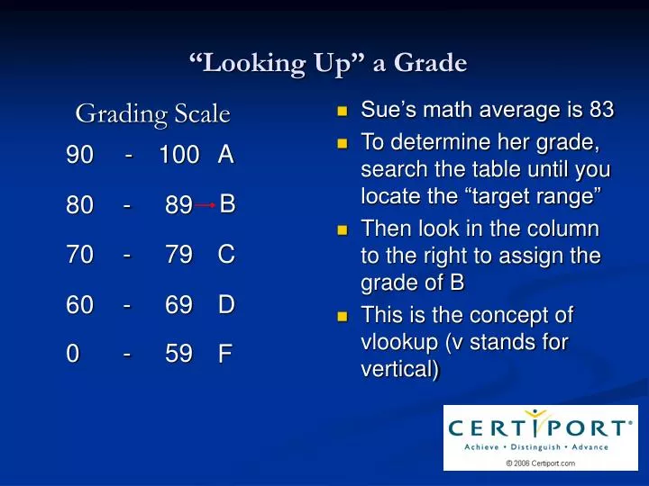
Grading Scale. Sue’s math average is 83 To determine her grade, search the table until you locate the “target range” Then look in the column to the right to assign the grade of B This is the concept of vlookup (v stands for vertical). “Looking Up” a Grade. VLOOKUP.

E N D
Grading Scale Sue’s math average is 83 To determine her grade, search the table until you locate the “target range” Then look in the column to the right to assign the grade of B This is the concept of vlookup (v stands for vertical) “Looking Up” a Grade
VLOOKUP • Excel’s VLOOKUP works in a similar manner • Like using a phone book, VLOOKUP begins searching down the first column in a vertical table, finds a specific row in that table, and pulls a value from another column in that row • VLOOKUP can locate and return the values efficiently and accurately
Use only the smallest number in each range Drop the extended portion of the range About the Lookup Table
More about the lookup table • The first column of the table should be in ascending order(lowest to highest) • The table is now ready for the vlookup function
The 1, 2, 3 of VLOOOKUP =vlookup(lookup_value,table_array,col_index_num) #1 #2 #3 What to look up Where to look (table range) The column # of the value to be returned Cell address of the value to look up (Sue’s 83 average) Grade Table 0 F 60 D 70 C 80 B 90 A Col 1 0 60 70 80 90 Col 2 F D C B A
#1 #2 #3 Where to look =vlookup( A6, $D$11:$E$15, 2) What to look up Enter vlookup formula in cell B6 Excel “looks for” the value in cell A6. 83 95 68 79 Col 2 0 F Excel searches down the first column of the table range “looking for” 83. As soon as it finds a number greater than the lookup value (83), it returns to next lowest value. Does not need to be an exact match. Use absolute cell addresses ($ signs in the table range) to keep the table range reference the same when the formula is copied. Excel pulls the value from Column #2 and places it in the active cell. 60 D 70 C target B 80 B 90 A Table Range $D$11:$E$15
What value will be looked up for Betty? #1 #2 #3 =vlookup( A7, $D$11:$E$15, 2) copied formula B 83 95 68 79 Where is Excel going to look for this value? 0 F 60 D 70 C 80 B 90 A A Which column on this row will be returned to the cell? Table Range
The lookup function is copied to all remaining cells. =vlookup( A6, $D$11:$E$15, 2) =vlookup( A7, $D$11:$E$15, 2) A 95 formula copied =vlookup( A8, $D$11:$E$15, 2) D 68 =vlookup( A9, $D$11:$E$15, 2) 79 C 0 F 60 D Absolute Cell Addresses 70 C Relative Cell Addresses 80 B 90 A $ sign before the column letter and row number keeps the table range the “same” from row to row when the formula is copied “What to look for” changes on each row.
$D$11:$E$15 This formula has been copied to Cell C8. What’s wrong with this formula? Use $ signs in the table range =vlookup( A8, D13:E17, 2) B 83 A 95 D #N/A 68 79 0 F 60 D Since no $ signs were used in the table range, the cells adjusted when the formula was copied. 70 C 80 B D13:E17 90 A A Empty Rows As a result #N/A appears in the cell.
grades Instead of using absolute cell addresses for the table range you can “name” the range =vlookup(A6,$D$11:$E$15,2) To create a named range, select the cells in the table, then click in the Name box andtype a name for the cells (no spaces are allowed) =vlookup(A7,$D$11:$E$15,2) A 95 =vlookup(A8,$D$11:$E$15,2) D 68 =vlookup(A9,$D$11:$E$15,2) 79 C 0 F If the grading table were given the named range of grades, the formula would be: =vlookup(A6,grades,2) =vlookup(A7,grades,2) =vlookup(A8,grades,2) =vlookup(A9,grades,2) 60 D 70 C 80 B 90 A D11:E15 = grades
VLOOKUP WIZARD • Click the Insert Function button (fx) on formula bar → Lookup & Reference category → VLOOKUP • Enter the values • Range_lookup is not bold (means it is not required) • TRUE (blank) is the default • finds the nearest value that is <= lookup value • FALSE • looks for an exact match • specific item A6 $E$11:$D$15 2
Lookup Table Locations • VLOOKUP can be used to “pull” information from an existing table • Same sheet • Separate sheet • Different workbook
Requires an exact match =VLOOKUP(A3,$A$12:$D$139,4,FALSE) Lookup table stored on same sheet
=VLOOKUP(A3,Employees!$A$12:$D$139,4,FALSE) Lookup table stored on a separate sheet named Employees
=VLOOKUP(A3,C:\[DistrictInfo]Employees!$A$12:$D$139,4,FALSE) Location [File Name] Sheet! Table Range Lookup table is stored in a different file on a sheet named Employees
Practice File Hands-on application practice exercises are included in the vlookup practice file.