Download
1 / 32
340 likes | 552 Views
The Grey Zone Project. Grey Zone committee: Andy Brown, Jeanette Onvlee, Martin Miller, Pier Siebesma. Introduction on the Grey Zone (from a parameterizational point of view) A proposal (thanks to Paul Field and Adrian Hill (Met Office)) Discussion and Next Steps. Pier Siebesma.

E N D
The Grey Zone Project Grey Zone committee: Andy Brown, Jeanette Onvlee, Martin Miller, Pier Siebesma • Introduction on the Grey Zone (from a parameterizational point of view) • A proposal (thanks to Paul Field and Adrian Hill (Met Office)) • Discussion and Next Steps Pier Siebesma
Motivation • Increased use of (operational) models in the “grey zone” (Dx = 1 ~10km) • Models operating in this resolution range resolve some of the “aggregation of convective cells” but certainly no individual convective cells. • This leads to the “wrong” perception that these “grey-zone” models, when operating without (deep) convection parameterizations, can realistically represent turbulent fluxes of heat, moisture and momentum. • Hence there is a urgent need of a systematic analysis of the behavior of NWP models operating in the “grey-zone”: • “The Grey Zone Project”
Some Background “Many of the parameterization issues (especially clouds and convection) evolve around finding the subgrid (co)variances of w, T and q”
Prime Example: Cloud schemes “Many of the parameterization issues (especially clouds and convection) evolve around finding the subgrid (co)variances of w, T and q”
qt qsat Prime Example: Subgrid Cloud Fraction “Many of the parameterization issues (especially clouds and convection) evolve around finding the subgrid (co)variances of w, T and q”
qsat(T) . (T,qt) qt T Prime Example: subgrid cloud fraction “Many of the parameterization issues (especially clouds and convection) evolve around finding the subgrid (co)variances of w, T and q”
qsat(T) . (T,qt) qt T Prime Example: subgrid cloud fraction “Many of the parameterization issues (especially clouds and convection) evolve around finding the subgrid (co)variances of w, T and q” Cloud fraction:
qsat(T) . (T,qt) qt T Prime Example: subgrid cloud fraction “Many of the parameterization issues (especially clouds and convection) evolve around finding the subgrid (co)variances of w, T and q” Cloud fraction:
This biased errors slowly go away if resolution increases: • Typically allowed for Dx~100m, i.e. at the LES scale • So for all models operating at a coarser resolution additional information about the underlying Probability Density Function (pdf) is required of temperature, humidity (and vertical velocity). • Or, as a good approximation, the variances and covariances: As a function of the used resolution!!
Example:a posteriori coarse graining • Use a reference (LES) model that resolves the desired phenomenum ( Dx << lphen) • Has a domain size much larger than the desired phenomenum ( L >> lphen) • Coarse grain the (co)variances across these scales subgrid resolved
Methodology: • Use a reference (LES) model that resolves the desired phenomenum ( Dx << lphen) • Has a domain size much larger than the desired phenomenum ( L >> lphen) • Coarse grain the (co)variances across these scales subgrid resolved l = L l = Dx
Applied to shallow cumulus convection: Subgrid contribution Subgrid contribution starts to shrink if l~ 5 lphen~5km l
Similar analysis for fluxes (heat flux) Grey zone sets in at smaller scales Due to the fact that the w-spectrum peaks at smaller scales
Not completely unrelated to stochastic physics……….. subgrid resolved l=1.6km l=6.4km l=12.8km Moisture turbulent flux
Stratocumulus generates larger horizontal scales……. How large is large enough? De Roode et al: JAS 61 p403 2004
Subgrid contribution Now the grey zone sets in at 10 km or more.
Schematics of the grey zone (including the stochastic arena) • Remarks: • The grey zone depends on the size of the considered process (convection (shallow or deep) , clouds (stratocumulus, shallow or deep) • The stochastic arena is stretching out a factor of 5 to 10 further. Deterministic (statistical) Arena Stochastic Arena Grey zone variance, flux total parametrized resolved Lphen 10~50 Lphen Horizontal resolution (Dx)
Proposal (from WGNE 2010 meeting) • Project driven by a few expensive experiments (controls) on a large domain at a ultra-high resolution (Dx=100~500m) (~2000x2000x200 grid points). • Coarse grain the output and diagnostics (fluxes etc) at resolutions of 0.5, 1, 2, 4, 8, 16, 32 km. (a posteriori coarse graining: COARSE) • Repeat CONTROLS with o.5 1km, 2km, 4km, 8km, etc without convective parametrizations etc (a priori coarse graining: NOPARAMS) • Run (coarse-grain) resolutions say 0.5, 1km, 2km, 4km and 8km with convection parametrizations (a priori coarse graining: PARAMS) • Preference especially from the mesoscale community for a cold air outbreak
Aims • Show how faithfully fluxes, variances, cloud structures, etc can be represented by comparing COARSE, NOPARAMS and PARAMS depending on all aspects of set-ups. • Guide improvements in current schemes especially at these resolutions - essential for future progress • Gain some insight and understanding of what can be achieved without parametrizations • Clarify what cannot/should not be done without parametrization also!! Strong Support from both the international NWP and Climate community
CONSTRAIN – proposal for cold air outbreak case(thanks to Paul Field & Adrian Hill, Met Office)
CONSTRAIN • flights over the North Atlantic from January 12 to 31 2010. • The proposed case is based in observations and NWP data from January 31st 2010. • Observations show that this day is characterised by northerly flow and stratocumulus clouds at 65N -10W. As air advects over warmer seas the Sc transitions to mixed-phase cumulus clouds at around 60N, prior to reaching land
The Case (1) • The Mesoscale Community is interested to start with an extra-tropical case • Cold-air outbreaks are of general interest for various communities • Proposal: “Constrain” cold-air outbreak experiment • 31 January 2010 • Participation of global models, mesoscale models but also from LES models !! • Domain of interest: 1500X1000 km • Quick Transition : ~ 12 hours
The Case (2) 4 Different Flavours • Global Simulations (at the highest possible resolution up to 5 km) • Mesoscale Models (Eulerian) • At various resolutions (up to ?) • Mesoscale Models (Lagrangian) • Idealized with periodic BC • highest resolution (~100m) • LES models (Lagrangian) • (in the same set up as 3)
LAM simulation Quasi-lagrangian trajectory Low cloud fraction
Quasi-lagrangian timeseries start point 65 N -10 W, 0 UTC
Initial Proposal for LES/Mesoscale Langrangian set-up • x,y domain = 250 X 250 km (how large is large enough? ) • dx, dy ~ 250 m • z domain = 5 km • dz = 20 m between surface up to 100m at 5000m • The case is initialised with total water, potential temperature based on output from the NWP simulation
Forcing Surface forcing Subsidence x hours spin-up with fixed SST
Discussion Points (1) • Global Model runs: • The cloud types under consideration are probably to small to be able to penetrate into the grey zone (at least for the turbulent fluxes) • So for these models it is more a classic parameterization excerise • Still relevant enough? • Look for (larger) cloud types for which the grey zone issues are more relevant? • MJO case , now? In a later phase? • Eulerian (operational) Mesoscale Model runs • Can some of these models reach the fully resolved mode “LES (~250m) implying a domain size of 1000X1500 km ? (4000X6000 grid points) • Will each mesoscale model run with the same lateral boundary conditions?
Discussion Points (2) • Lagrangian runs (LES and Mesoscale) • How large is large enough? (250X250km) • How long do we need to spin up in order to let mesoscale structures form • How much do we constrain/simplify the case in the Lagrangian mode: • simplify subsidence fields? • Prescribe drag coefficients for the surface fluxes? • Nudge winds?
Time Line and Organisation • october/december : testruns with at least 2 LES (MOLEM, DALES) • Release January 2012 Organisation: different case leaders for the 4 flavours ( a la TWP-ICE)? MPI has shown interest (Verena Grutzun) Meto? Others?