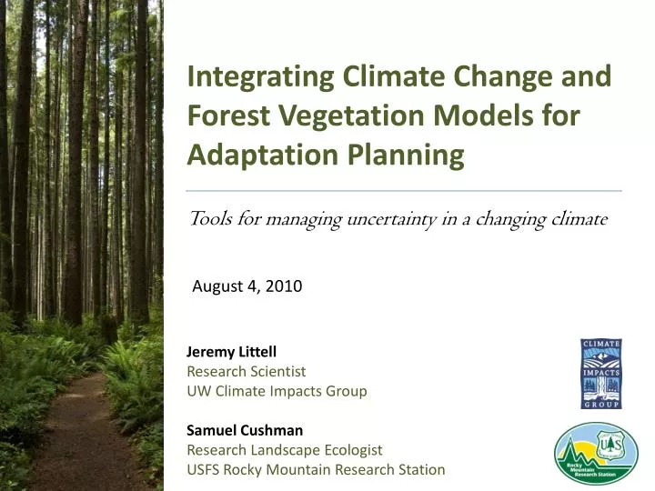
Integrating Climate Change and Forest Vegetation Models for Adaptation Planning

1. Integrating Climate Change and Forest Vegetation Models for Adaptation Planning August 4, 2010 Tools for managing uncertainty in a changing climate Jeremy Littell Research Scientist UW Climate Impacts Group Samuel Cushman Research Landscape Ecologist USFS Rocky Mountain Research Station

2. Acknowledgements This webinar is sponsored and jointly hosted by the USFS Western Wildland Environmental Threat Assessment Center (WWETAC). Special thanks to Charles (Terry) Shaw at WWETAC for his efforts. Climate Science in the Public Interest Material for the webinar is based on the paper: Littell, J.S., B.K. Kerns, S. Cushman, D. McKenzie, and C. Shaw. 2010. On using climate driven ecological models to inform decision making to prepare for climate change. In prep.

3. Webinar Tips • Mute phones to reduce background noise (*6 or “mute” button). • Questions can be entered in the chat box (lower left) during the webinar. Chat box and telephone questions will be answered during the Q&A session. • Can use “Full Screen” option for larger screen view • Additional opportunities for Q&A: • Post-presentation Q&A session (11:00-11:30) • Email CIG: cig@uw.edu • Presentation will be posted at: http://cses.washington.edu/cig/outreach/webinars/vegmodel710.shtml http://www.fs.fed.us/wwetac/workshops/webinar/clim_veg_model_webinar.pdf

4. Adaptation Challenges • Climate is changing and impacting many ecosystem components. • Past experiences will be a less useful guide to future conditions. Key climate impact pathways

5. Adaptation challenges cont’d • Many present-day planning decisions have time horizons that will be affected by climate change. • Combining climate models with vegetation models can help better define plausible future conditions. Use in planning has been limited, however: • Decision makers have limited experience with models, model output, and integrating output into decision making processes; • Developing scenarios can be expensive (both in terms of time and $) and therefore require tradeoffs when implementing; and • Integrating vegetation models and climate models brings a new level of complexity to traditional modeling activities.

6. Adaptation Planning The goal is to use best available science to: • Inform understanding of current priorities and vulnerability to climate change; • Evaluate how climate change will impact those priorities; and • Develop management strategies for increasing resilience of priorities given likely impacts. But, at what scale, and with which tools??

7. Webinar Objectives Review key considerations for: • Selecting greenhouse gas emissions scenarios and climate models, • Integrating climate scenarios in vegetation modeling, and • Some considerations in applying modeling output for adapting to climate change. Review key sources of uncertainty in climate and vegetation modeling and how these are addressed in model/scenario selection.

8. Global Climate Models (GCMs) • More than 20 GCMs developed by modeling centers around the world. • GCMS break the world into large (~60 to 180 miles) grid sizes and model complex interactions between the atmosphere, ocean, etc. within each grid cell. Adapted from http://www.ucar.edu/news/releases/2004/images/CLIMATE8.gif

9. Global Climate Models (GCMs) cont’d • GCMs respond differently to the same emissions because they have different ways of characterizing components of the climate system, including: • sensitivity to greenhouse gas concentrations; • how physical processes that affect climate are constructed and described (e.g., viscosity of the ocean); • how feedbacks between the processes are modeled (e.g., how fast the ocean warms once ice cover diminishes past a certain point) • Some things are common to most or all models; others are treated differently from model to model. After Henderson-Sellers and McGuffie, 1987 http://www.geosc.psu.edu/~dbice/DaveSTELLA/climate/climate_modeling_1.htm NCAR Mote et al. 2008

10. The differences between models are one of the larger sources of uncertainty in generating climate data Example: Model comparison for observed (20th century) PNW temperature trend 1900-1999 trend – USHCN (C°) Mote and Salathé, 2009

11. Approaches to Choosing Climate Models for Regional Purposes NASA Earth From Space (SeaWiFS) Example: 18 GCMs • All models are equally plausible. • Average all 18 models together = ensemble Ensemble • 2. All models are equally plausible, but • We want to plan for a range of scenarios. • Select “bracketing” models Warmest Coolest • 3. Some models perform better than others. • Select best performing models for ensemble - Driest Filter 18 models based on performance criteria: trend, pressure, means, etc Modified from original image: www.psdgraphics.com Ensemble Wettest

12. Greenhouse Gas Emissions Combine different estimates of population growth, technology development, energy sources (e.g., fossil fuels vs. “green” energy), etc. Model Range Emissions Temperature change Source: IPCC AR4 Summary For Policy Makers

13. Choosing Greenhouse Gas Emissions Scenarios • No one emissions scenario is considered more likely than another. • Choice of scenarios is in large part a function of risk management: are you risk tolerant vs. risk averse? • Alternative : Model the “ensemble mean” of multiple climate models for one to a few emissions scenarios (B1, A1B, A2) • Advantage: helps address computational limitations; reduces influence of internal model variability in any single model • Disadvantage: Future may not look like the “mean”; natural variability in the climate system diminished by using only the mean change

14. A Note About Timing and Emissions Differences in scenarios, and thus changes in climate and related impacts, do not strongly diverge until after mid-21st century. IPCC 2007 Projected Warming for the Pacific Northwest Mote and Salathé 2009 This is true at the global scale and, as a result, at the regional scale as well.

15. Choosing GCMs/Scenarios • Are multiple scenarios and multiple GCMs needed for impacts modeling, or is an ensemble mean sufficient?

16. Choosing GCMs/Scenarios • Are multiple scenarios and multiple GCMs needed for impacts modeling, or is an ensemble mean sufficient? • 2. Do the models and emission scenarios selected match the risk framework (risk tolerant vs. risk averse)?

17. Choosing GCMs/Scenarios • Are multiple scenarios and multiple GCMs needed for impacts modeling, or is an ensemble mean sufficient? • 2. Do the models and emission scenarios selected match the risk framework (risk tolerant vs. risk averse)? • Do the models chosen have good fidelity to 20th century observations using a regional focus?

18. Choosing GCMs/Scenarios • Are multiple scenarios and multiple GCMs needed for impacts modeling, or is an ensemble mean sufficient? • 2. Do the models and emission scenarios selected match the risk framework (risk tolerant vs. risk averse)? • Do the models chosen have good fidelity to 20th century observations using a regional focus? • 4. Is the spatial and temporal scale of the climate information appropriate to planning or decision making?

19. Scale and Statistical Downscaling Global climate models do not project climate at a scale as fine as we would like for impacts studies, so we “downscale” them. ~200 km (~125 mi) resolution ~5 km (~3 mi) resolution

20. Scale and Statistical Downscaling To do this we: • Take historical climate and map it to a grid (~ 3.5 mi) • Compare each grid cell to a climate model’s grid cell (~ 100 mi) • Use the difference between them to adjust the future projections at the same coarse grid

21. Downscaling Methods • Different applications have driven the development of downscaling methods. • The method you choose should be informed by the process you are trying to understand in the future. • Two general approaches: -- Statistical downscaling (e.g., composite delta, BCSD,hybrid delta) -- Dynamical downscaling (i.e., Regional Climate Modeling)

22. Downscaling Methods: Statistical Downscaling • Composite delta: Simple, easy to explain “snapshot” of average future conditions. • Suitable when you want to know the mean change at a monthly time step. • Ex: Changes in future vegetation distribution by biomes

23. Downscaling Methods: Statistical Downscaling • Composite delta: Simple, easy to explain “snapshot” of average future conditions. • Suitable when you want to know the mean change at a monthly time step. • Ex: Changes in future vegetation distribution by biomes • Bias Corrected and Spatially Downscaled (BCSD): Produces a transient (i.e. continually varying) daily time series. • Suitable when you want to model the change in variability around monthly mean, changes in extremes at a monthly time step, or frequency of extreme events. • Ex: Changes in phenology Other methods that pull features from both methods (e.g., hybrid delta) are available

24. Downscaling Methods: Dynamical Downscaling (Regional Climate Modeling) Advantages: • Modeling of the climate system at finer spatial scales (5-50 km, or 3-32 mi resolution); • Can represent major topographic features, land surface effects; • Can simulate small extreme weather systems. Disadvantages: • Computationally demanding • Adds to uncertainty from GCMs - GCMs constrain outcomes Suitable for processes driven by local feedbacks.

25. Caveat on Scale • A finer scale does not necessarily mean the projections are more realistic or better constrained. • Generally, all methods can be stepped down from the monthly to a daily or finer time step but you have to make certain assumptions that can add to uncertainty. • Additional key questions: • Is more to be gained by finer downscaling? • Is it worth the additional cost and potential uncertainty? • How does the scale of information match the detail of the ecosystem impact model being used?

26. Empirical Climate Interpolation

27. Aug. Tmin Mar. Tmin Observed (C) Predicted (C) Sep. Precip Jun. Precip Predicted (mm) Observed (mm)

28. Limitations of Interpolated Climate Models • Current methods of predicting temperatures in mountains rely on existing weather stations • Most stations located in cities, valleys and at low elevations, so we have to interpolate. • DAYMET uses constant lapse rate (6.5 deg C/1000 meters); PRISM is refining lapse • Thin plate spline models (e.g. ANUSPLIN) fit the data to elevation locally, using differences between nearby stations.

29. Challenges of Predicting Temperatures in Complex Topography Variations in temperature variability are known to exist, but are not captured by current models. • Variable lapse rates • Cold air pooling at night • Mid-slope thermal belts • Inversions

30. Temporal and Spatial Variability in Nocturnal Air Temperatures in Two North Idaho Mountain RangesHolden, Cushman, Crimmins and Littell in review

31. Temperature is not always a function of elevation Daytime Temp (C) 14.6 8.5 Higher elevations = cooler Ridge top (moderate) Valley mid slope = warmer Valley floor (moderate)

32. Temperature is not always a function of elevation Nighttime Temp (C) 12.7 6.3 Higher elevation canyon = much cooler Valley floor (moderate) Valley mid slope = warmer

33. Incorporating Climate Info into Vegetation ModelsImplicit and Explicit Models Climate information can be incorporated into ecosystem impacts models explicitly or implicitly. • Explicit models: climate is a direct predictor of an ecosystem response. Direct relationships reduce uncertainty. • Implicit models: climate impact on ecosystem response is indirect (e.g., model predictors are elevation, lat/long, or site index, not temp or precip directly)

34. Scale and Modeling Approaches stand watershed region • Mechanistic • Empirical • Stochastic year decades centuries Approaches focus on specific scales in time and space. Bob Keane

35. Stand Watershed Region FOFEM FARSITE NWS Models Consume Burnup Year Flammap RCM’s SIMPPLLE FETM FVS Decades Gap Models CRBSUM RMLANDS Gap Models Centuries MAPPS Landis FOREST-BGC DGVM’s LANDSUM Bob Keane

36. Statistical Species Distribution Models Goals: • Develop predictive models that relate species distributions with their climatic drivers • Use models to extrapolate future potential species distributions based on future climate projections Current GDD > 5C 2090s B2 GDD > 5C P. Ponderosa current P. Ponderosa 2090s Rehfeldt et al. 2006, http://forest.moscowfsl.wsu.edu/climate/plantDistributions.html

38. Predicting Shrub Species Distributions with Topoclimatic Data in Complex TerrainHolden, Cushman, Evans, submitted.

39. Statistical Species Models Strengths Limitations Some methods numerically difficult Ecological controls on species distributions not considered explicitly Physical and physiological processes responsible for relationships not modeled explicitly* *Future projections assume these are captured in statistical relationships that are the same as in the past • Conceptually simple • Explicit incorporation of climate and implicit individualistic response of species • Validation probabilistic and expression of model error quantitative

40. Gap Models Goals: • Develop process models that describe stand development as growth of individual trees • Use models to extrapolate stand composition, tree growth, mortality, structure as a function of stand state and limiting factors including climate Shugart and Noble, 1981

41. Gap Models Strengths Limitations Require local calibration; limits use by managers Most gap models are not spatially explicit Ecophysiology is limited compared to BGC models Not prognostic for shorter term analysis of response to management interventions • Individual tree and stand level provides detailed response applicable to management problems • Can be linked to spatially-explicit landscape scale models • Include physiological processes that can be linked to climate drivers explicitly

42. Forest Vegetation Simulator (FVS) FVS is an individual-tree, semi-distance-independent growth model. Inputs include an inventory of site conditions and a set of measurements on a sample of trees (e.g., tree size, species, crown ratio, recent growth and mortality rates). Outputs include summaries of tree volume, species distributions, and growth and mortality rates that are often customized for specific user needs. Spatial scales range from a single stand to thousands of stands. The temporal scale has traditionally been about 200 years (400 years maximum)

43. Forest Vegetation Simulator (FVS)

44. Climate “Smart” FVS Addressing Climate Change in the Forest Vegetation Simulator to Assess Impacts on 1 Landscape Forest Dynamics --- Crookston et al. in press Forest Ecology and Management • Forest Vegetation Simulator (FVS) adjusted to account for expected climate effects. • This was accomplished by: • Adding functions that link mortality and regeneration of species to climate variables • Constructing a function linking site index to climate and using it to modify growth rates • Adding functions accounting for changing growth rates due to climate-induced genetic responses.

45. Biogeochemical Models Goals: • Develop process models that describe earth system biogeochemical cycles (e.g., carbon, nitrogen) – but , necessarily, also vegetation (forest) productivity • Use models to extrapolate future pools of carbon as a function of plant photosynthesis, respiration, which are in turn functions of nitrogen, water, energy BIOME-BGC www.ntsg.umt.edu/models/ bgc/images/bgcflow.png Numerical Terradynamic Simulation Group Graphic: W. Parton

46. Biogeochemical Models Strengths Limitations variables used by managers (e.g., stand structure) are not available or are limited sensitive to downscaling: some processes operate at very small scales OR are generalized (applies to other model classes as well) • track climate controlled processes (e.g., hydrology, gas exchange) in forests and account for their interactions • carbon budgets are a natural component • ecosystem process focus makes them flexible for different vegetation types • can identify process- and rate-limiting factors in different regions

47. LandscapeVegetation Models Goals: • Model spatially dependent and spatially contagious processes at multiple scales • Use models to extrapolate future vegetation structure, disturbance interactions, in real world complex topography Source: Cushman et al 2008 Source: D.Urban

48. Disturbances Simulated Eric Gustafson

49. Spatial Dynamism: How spatially dependent processes are modeled Eric Gustafson

50. Strengths & limitations of various LDSMs • VDDT/TELSA • Relatively easy to use, flexible, portable, conceptually simple • Less scientific & analytical rigor, limited dynamics. • LANDSUM • Minimal inputs, flexible, portable • Does not use spatial context, limited spatial dynamism except for fire • RMLANDS • High spatial dynamism, good analytical capabilities • Computationally intensive, requires high level of developer support, documentation limited Eric Gustafson