Download

1 / 34
340 likes | 467 Views
Trends in Maximum and Minimum Temperature Deciles in Select Regions of the United States. By Rebecca Smith Melissa Griffin Dr. James O’Brien. Outline. Purpose and Background Data and Quality Control Understanding the Decile Plot Statistical Analysis Regional Analysis Station Analysis

E N D
Trends in Maximum and Minimum Temperature Deciles in Select Regions of the United States By Rebecca Smith Melissa Griffin Dr. James O’Brien
Outline • Purpose and Background • Data and Quality Control • Understanding the Decile Plot • Statistical Analysis • Regional Analysis • Station Analysis • Identifying variable periods in time • Identifying long-term trends • Conclusions and Future Work
Purpose • To better analyze temperature trends by evaluating shifts in maximum and minimum temperatures using decile maps • To examine the region for patterns in trends at each decile • To properly explain why trends are occurring where and when they are occurring
Purpose • To better analyze temperature trends by evaluating shifts in maximum and minimum temperatures using decile maps • To examine the region for patterns in trends at each decile • To properly explain why trends are occurring where and when they are occurring
Background: Methods of Examining Trends • Generic Studies--One annually and globally averaged temperature • Is this representative of any point on the globe at any given time? • Regional or station annual and seasonal averages • Mitchell (1953) used annual and seasonal mean temperatures at 77 U.S. stations • Kalnicky (1974) used U.S. Weather Bureau stations to calculate annual and seasonal deviations
Background: Methods of Examining Trends • Monthly averaged • Hansen et al. (2001) and Kalnay et al. (2006) averaged daily max and min temperatures, then averaged over a month • Hale et al. (2006) calculated monthly averages, plus monthly max and monthly min • Tails of the Distribution • DeGaetano and Allen (2002) and Peterson et al. (2007) examined the number of temperature extreme days over a threshold (e.g. 10% and 90%)
Data • National Weather Service Cooperative Station Network • Records daily maximum and minimum temperatures and precipitation • Station Requirements • Located in midwestern, southern, and mid-Atlantic states • Period of record 1948-2004 • Less than 10% missing data (~5 years)
Missing Data • Multiple Linear Regression technique used to replace missing data • 2 to 5 neighboring stations within 50 miles of reference station chosen • Residuals calculated by removing trend and the seasonal cycle from the raw data • Correlations between reference residual and surrounding residuals are computed
Missing Data • Multiple linear regression line calculated using residuals • Regression line used to replace missing data values with an estimated residual • Trend and seasonal cycle added back to the estimated residual
Statistical Analysis: t-test Standard Deviation, where: and t-statistic accepts or regects the null hypothesis, H0. H0 = the calculated slope is 0. If H0is rejected, then the slope is significantly different than 0. This value is compared to a critical t value, tcrit, found by calculating degrees of freedom when autocorrelation of T first goes to zero. tcrit value is based on a 95% confidence interval t-statistic:
Statistical Analysis: Bootstrapping • Randomly pick 10 years out of 57-year period • Sort the years • Calculate the slope based on corresponding temperature data • Bootstrap 1000 times for each decile • Sort 1000 slopes in ascending order • Assume 95% confidence interval • 975th slope is top threshold • 25th slope is bottom threshold • Average of 1000 slopes should be close to actual slope
Regional Analysis • Primarily cooling in maximum temperature deciles • Much more variability in minimum temperature deciles, but more warming than cooling • Some studies have shown a decrease in the annual temperature range (Peterson et al, 2007 and Kalnay et al, 2006) • Decile analysis shows a decrease in the diurnal temperature range
Station Analysis • How do cool periods or warm periods in different seasons show up on the decile plot?
Station Analysis • Indianapolis National Weather Service climatology page coldest winters on record: • 1976-1977 • 1977-1978 • Entire state experienced especially cold winters in the late 1970s • This clearly shows up in the decile plots
Station Analysis • Very warm period in early 1950s associated with severe drought conditions over much of the U.S. • NCDC states that summer temperatures were some of the hottest recorded
Station Analysis • Let’s analyze how long term trends appear on the decile map…
Analysis: Columbus, GA • Station located at the airport • Airport just northeast of central Columbus • Designated land cover for station is urban • Muscogee County population increased by over 50% from 1950 to 1990 • Could urban growth have an effect on decile temperature trends?
Analysis: Columbus, GA • Uniform land cover throughout the region • Urban effects would cause local warming • Is station warming more than the other stations nearby? Columbus and its surrounding stations for 1st decile minimum temperatures
Summary and Conclusions • Decile maps provide a fresh look at station temperature data • Allows for a complete “snapshot” for the entire distribution of temperatures • Regional analysis shows significant cooling in the maximum temperatures • Minimum temperatures more variable, but dominated by significant warming • This suggests a decrease in the DTR
Summary and Conclusions • Variability in wintertime temperatures shows up in the lower deciles • Variability in summertime temperatures shows up in the upper deciles • Long term trends are easy to identify on decile plots • Statistical testing can provide helpful information for each decile
Continued Work • Thesis work • How station dynamics affect the observed temperature trends (Apalachicola, FL) • Identifying regional or local trends and what is causing them (field significance testing) • For publication and website • Decile maps will be created for the rest of the country’s COOP stations • To view and download decile maps: http://gis.coaps.fsu.edu/httpdocs/climstudy.php
Questions? To view and download decile maps: http://gis.coaps.fsu.edu/httpdocs/climstudy.php