Download

1 / 48
480 likes | 482 Views
This chapter discusses the implementation of evolutionary computation techniques such as genetic algorithms and particle swarm optimization. It covers issues related to representation, adaptation, and algorithm design. Several benchmark functions are used to demonstrate the effectiveness of these techniques.

E N D
Evolutionary Computation Implementations: Outline • Genetic Algorithm • Mainly a canonical version • Crossover: one-point, two-point, uniform • Selection: Roulette wheel, tournament, ranking • Five benchmark functions • Particle Swarm Optimization • Global and local versions • Multiple swarm capability • Same benchmark functions as GA plus three for constraint satisfaction
EC Implementation Issues (Generic) • Homogeneous vs. heterogeneous representation • Online adaptation vs. offline adaptation • Static adaptation versus adaptive adaptation • Flowcharts versus finite state machines
Homogeneous vs. Heterogeneous Representation • Homogeneous representation • Used traditionally • Simple; can use existing EC operators • Binary is traditional coding for GAs; it’s simple and general • Use integer representation for discrete valued parameters • Use real values to represent real valued parameters if possible • Heterogeneous representation • Most natural way to represent problem • Real values represent real parameters, integers or binary strings represent discrete parameters • Complexity of evolutionary operators increases • Representation-specific operators needed
Binary Representations • Advantages • Simple and popular • Use standard operators • Disadvantages • Can result in long chromosomes • Can introduce inaccuracies
Final Thoughts on Representation • The best representation is usually problem-dependent. • Representation is often a major part of solving a problem. • In general, represent a problem the way it appears in the system implementation.
Population Adaptation Versus Individual Adaptation • Individual: Most commonly used. Pittsburgh approach; each chromosome represents the entire problem. Performance of each candidate solution is proportional to the fitness of its representation. • Population: Used when system can’t be evaluated offline. Michigan approach: entire population represents one solution. (Only one system evaluated each generation.) Cooperation and competition among all components of the system.
Static Adaptation Versus Dynamic Adaptation • Static: Most commonly used. Algorithms have fixed (or pre-determined) values. • Adaptive: Can be done at • Environment level • Population level (most common, if done) • Individual level • Component level Balance exploration and exploitation.
Flowcharts Versus Finite State Machines • Flowcharts: Easy to understand and use. Traditionally used; best for simpler systems • Finite State Machine Diagrams: Used for systems with frequent user interaction, and for more complex systems. More suited to structured systems, and when multi-tasking is involved.
Handling Multiple Similar Cases • If two possibilities, use if-then • If three or more, use switch (with cases); or function pointer (order is critical)
Allocating and Freeing Memory Space • Arrays and vectors should be dynamically configured • Allocate memory: calloc • Release memory: free
Error Checking • Use frequently • Use to debug • Can use assert() [remove when program debugged]
Genetic Algorithm Implementation • Essentially a canonical GA that utilizes crossover and mutation • Uses binary representation • Searches for optima with real value parameters • Several benchmark functions are included
Data Types Enumeration data type used for selection types, crossover types, and to select the test function. C has no data type for ‘bit’ so used unsigned character type for population. A bit (or a byte) can represent a bit; computational complexity issues must be addressed.
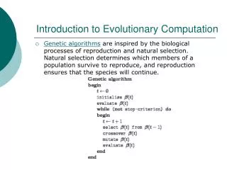
The GA main() Routine The GA_Start_Up routine: Reads in problem-related parameters such as the number of bits per parameter from the input file. Allocates memory Initializes population The GA_Main_Loop runs the GA algorithm: Evaluation Selection Crossover Mutation The GA_Clean_Up: Stores results in an output file De-allocates memory
GA Selection Mechanisms In ga_selection() routine • All use elitism • Proportional selection – roulette wheel that uses fitness shifting and keeps fitnesses positive • Binary tournament selection – better of two randomly-selected individuals • Ranking selection – evenly-spaced fitness values; then like roulette wheel
Mutate According to Bit Position Flag When 0, bit-by-bit consideration When 1, mutation done that is approximation of Gaussian Probability of mutation mb varies with bit position: where b=0 for the least significant bit, 1 for the next, etc. and m0is the value in the run file. Bit position is calculated for each variable. The mutation rate for the first bit is thus about .4 times the value in the run file. (This mutation is similar to that carried out in EP and ES (Gaussian).
Crossover Flag 0: One-point crossover 1: Uniform crossover 2: Two-point crossover
GA.RUN To run implementation: C>\ga ga.run result.dat 10 4 15000 16 20 0.75 0.005 0.02 0 2 1 result file name dimension function type 0: F6 1: PARABOLIC 2: ROSENBROCK 3: RASTRIGRIN 4: GRIEWANK maximum number of iterations bits per parameter population size rate of crossover rate of mutation termination criterion (not used in this implementation, but must be present) mutation flag 0: base mutation 1: bit position mutation crossover operator 0: one point; 1: uniform; 2: two point selection operator 0: roulette; 1: binary tournament; 2: ranking; Directory with ga.exe and run file
Result file: part 1 of 2 resultFile ..........................result function type .......................4 input dim ...........................10 max. No. generation..................15000 bits for eachPara....................16 boundary value.......................600.000000 popu_size............................20 individual length ...................160 crossover rate ......................0.750000 mutation rate ......................0.005000 term. criterion .....................0.020000 flag_m (1:bit position;0:cons) ......0 c_type (0:one,1:unif,2:two)..........2 selection type ......................1 generation: 15000 best fitness: -0.067105 variance: 22.179015
fitness values: fit[ 0]: -0.067105 fit[ 1]: -3.640442 fit[ 2]: -0.423313 fit[ 3]: -0.067105 fit[ 4]: -0.067105 fit[ 5]: -0.153248 fit[ 6]: -1.761599 fit[ 7]: -0.067105 fit[ 8]: -3.241397 fit[ 9]: -0.089210 fit[10]: -0.935671 fit[11]: -0.935671 fit[12]: -1.987072 fit[13]: -1.390572 fit[14]: -0.279645 fit[15]: -23.843609 fit[16]: -1.497647 fit[17]: -1.263834 fit[18]: -90.743202 fit[19]: -51.928169 parameters: para[ 0]: 3.140307 para[ 1]: 4.440375 para[ 2]: 5.410849 para[ 3]: 0.009155 para[ 4]: -7.003891 para[ 5]: -0.009155 para[ 6]: 8.194095 para[ 7]: 0.009155 para[ 8]: 9.365988 para[ 9]: -0.009155 begin time at: Mon Oct 01 08:35:14 2001 finish time at: Mon Oct 01 08:36:14 2001 Result file: part 1 of 2
PSO Implementation • Basic PSO as previously described is implemented first • A multi-swarm version (co-evolutionary PSO) is also implemented • The implementation is based on a state machine • Arrows represent transitions • Transition labels indicate trigger for transition • Can initialize symmetrically or asymmetrically
PSO Attributes • Symmetrical or nonsymmetrical initialization • Minimize or maximize • Choice of five functions • Inertia weight can be constant, linearly decreasing, or noisy • Choose population size • Specify number of dimensions (variables)
PSO State Machine • Nine states • A state handler performs action until state transition • State machine runs until it reaches PSOS_DONE
State Handling Routines • State handling routine called depends on current state • The routine runs until its conditions are met, i.e., the maximum population index is reached
PSO main()Routine • Simple • Startup: reads parameters, and allocates memory to dynamic variables • Cleanup: stores results and de-allocates memory
The Co-Evolutionary PSO • Can use for problems with multiple constraints • Uses augmented Lagrangian method to convert problem into min and max problems • One solves min problem with max problem as fixed environment • Other solves max problem with min problem as fixed environment
Co-Evolutionary PSO Procedure • Initialize two PSOs • Run first PSO for max_gen_1 generations • If not first cycle, evaluate the pbest values for second PSO • Run second PSO for max_gen_2 generations • Re-evaluate pbest values for first PSO • Loop to 2) until termination criterion met
Method of Lagrange Multiplier (Constraint Optimization) Example Suppose a nuclear reactor is to have the shape of a cylinder of radius R and height H. Neutron diffusion theory tells that such reactor must have the following constraint. We would like to minimize the volume of the reactor By using the equations above, then, By multiplying first equation by R/2 and the second by H, you should obtain
Co-Evolutionary PSO Example • 1st PSO: Population member is a vector of elements (variables); run as minimization problem • 2nd PSO: Population member is a vector of λ values [0,1]; run as maximization problem • Process: • Run first PSO for max_gen_1 generations (e.g., 10); fitness of particle is maximum obtained with any λ vector (λ values are fixed). • If not first cycle, re-calculate pbests for 2nd PSO • Run second PSO for max_gen_2 generations; optimize with respect to λ values in 2nd population; variable values are fixed. • Recalculate pbest values for first PSO. • Increment cycle count and go to 1. if not max cycles
Benchmark Problems • For all benchmark problems, population sizes set to 40 and 30 • 10 generations per PSO per cycle • Different numbers of cycles tested: 40, 80, and 120 • In book, linearly decreasing inertia weight used • 50 runs (to max number of cycles) done for each combination of settings
State Machine for Multi-PSO Version typedef enum PSO_State_Tag { PSO_UPDATE_INERTIA_WEIGHT, // Update inertia weight PSO_EVALUATE, // Evaluate particles PSO_UPDATE_GLOBAL_BEST, // Update global best PSO_UPDATE_LOCAL_BEST, // Update local best PSO_UPDATE_VELOCITY, // Update particle's velocity PSO_UPDATE_POSITION, // Update particle's position PSO_GOAL_REACH_JUDGE, // Judge whether reach the goal PSO_NEXT_GENERATION, // Move to the next generation PSO_UPDATE_PBEST_EACH_CYCLE,// Update pbest each cycle for //co-pso due to the //environment changed PSO_NEXT_PSO, // Move to the next PSO in the same cycle or // the first pso in the next cycle PSOS_DONE, // Finish one cycle of PSOs NUM_PSO_STATES // Total number of PSO states } PSO_State_Type;
PSO-Evaluate for Multi-PSOs For the co-evolutionary PSO, each PSO passes its function type to the evaluate_functions() routine to call its corresponding function to evaluate the PSO’s performance. For example, if the problem to be solved is the G7 problem, one PSO for solving the minimization problem calls G7_MIN(), and the other PSO for solving maximization problem will call G7_MAX().
G1 Problem where The global minimum is known to be x*= (1,1,1,1,1,1,1,1,1,3,3,3,1) with f(x*) = -15
For G1 Problem For both swarms, the function that is evaluated is the augmented Lagrangian.
Sample PSOS Run File, Part 1 2 # of PSOs 1 update pbest each cycle flag 300 total number of cycles to run 0 optimization type (0 = min, 1 = max) 0 function type (G1_min) 1 inertia update method (1 = linearly decreasing) 1 initialization (1 = asymmetric) 0.0 left initialization 50.0 right initialization 10 max velocity 100 max position 100 max generations per cycle 30 population size 13 dimensions 0.9 initial inertia weight 1 boundary flag (1 = enabled) 0 1.0 lower and upper boundaries for parameters (13 for G1) 0 1.0 0 1.0 0 1.0 0 1.0 0 1.0 0 1.0 0 1.0 0 1.0 0.0 100.0 0.0 100.0 0.0 100.0 0.0 1.0
Sample PSOS Run File, Part 2 Values for second swarm, as in part 1 1 1 = max 1 (G1_max) 1 1 0.0 1.0 0.5 1 70 20 9 0.9 1 0.0 1.0 0.0 1.0 0.0 1.0 0.0 1.0 0.0 1.0 0.0 1.0 0.0 1.0 0.0 1.0 0.0 1.0
Single PSO Run File (annotated) 1 num of PSOs 0 pso_update_pbest_each_cycle_flag (only for multiple swarms) 40 total cycles of running PSOs 0 optimization type: 0=min or 1=max 6 evaluation function (F6) 1 inertia weight update method: 1=linear decreasing 1 initialization type: 0=sym,1=asym -10.0 left initialization range 50.0 right initialization range 40 maximum velocity 100 maximum position 50 max number of generations per cycle 30 population size 2 dimension 0.9 initial inertia weight 0 boundary flag 0=disabled 1=enabled boundaries if boundary flag is 1 Evaluation functions 0: G1_MIN 1: G1_MAX 2: G7_MIN 3: G7_MAX 4: G9_MIN 5: G9_MAX 6: F6 7: SPHERE 8: ROSENBROCK 9: RASTRIGRIN 10: GRIEWANK