Download
1 / 29
300 likes | 426 Views
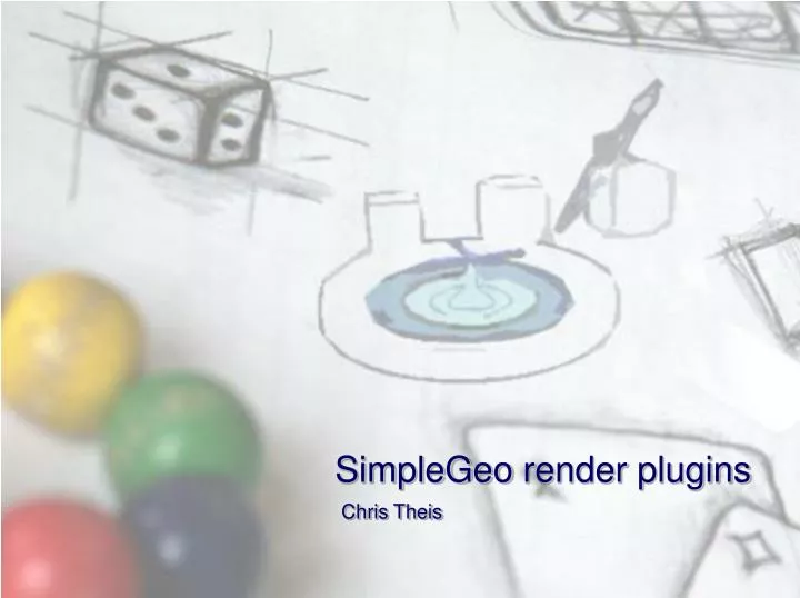
SimpleGeo render plugins. Chris Theis. SimpleGeo architecture. GIMLI Geometric input modeling language interface. SG-PLEX SimpleGeo plugin extensions. GUI Graphical user interface. Command manager. CSG – Engine. Importer/ Exporter. Proprietary Renderer. Portable Standard C++.

E N D
SimpleGeo render plugins Chris Theis
SimpleGeo architecture GIMLI Geometric input modeling language interface SG-PLEX SimpleGeo plugin extensions GUI Graphical user interface Command manager CSG – Engine Importer/ Exporter Proprietary Renderer Portable Standard C++ OpenGL B-Rep - Kernel
Plugins Plugins are extensions that can be loaded at runtime They can be used to • extend SimpleGeo’s proprietary renderer • act as 3rd party import/export filter • … They are contained in the file SGPluginsX.X.zip whichshould be unpacked into the SimpleGeo installation directory (recommended).
Available plugins DaVis 3D (see the demo in the videos directory) • reads FLUKA USRBIN, PHITS, XYZ, and GRIDCONV files • displays the binned data of up to 3 planes (XY,YZ,ZX) than can be interactively moved through the data set • data can be superimposed on top of geometry • the color tables are user configurable and interpolate if requested
SimpleGeo/DaVis3D Courtesy of E. Feldbaumer, H. Vincke
Data extraction Extraction of values(planes, profile functions or single bins)
Data extraction Profiles can be extracted taking 1 bin into account along the intersection of 2 planes statistical fluctuations Solution: “Averaged profiles”: (DaVis3D version >=3.5) an arbitrary averaging volume can be defined which is moved along the intersection and the resulting profile is extracted
Data post-processing • Question: • What’s the average dose • at a workplace? • Solution: • Rough estimate from the • 2D dose map (might not match in 3D!) • Foresee a geometric region in the input Courtesy of E. Feldbaumer, H. Vincke
Data post-processing Courtesy of E. Feldbaumer, H. Vincke • Alternative solution with • DaVis3D • Define arbitrary volume • interactively while browsing the data. • Calculate averages on-the-fly while • moving the volume through the data set
More post processing options The following post – processing options are available for FLUKA USRBIN files (ASCII format): • Averaging over several USRBIN results including error calculation • (inconsistent weights are treated accordingly) • Sum of several USRBIN results • Difference of 2 USRBIN results • Ratio of 2 USRBIN results • * Individual additional weights can be specified for each file.
Threshold detection Typical question: Where is the dose >1 mSv/h? Development of an automatic threshold contouring algorithm
Additional visualization modes Contour rendering Smoothed extrusion rendering
“Hands-on” example of DaVis 3D Hint: Creating copies of the *.plx files allows for loading Multiple instances of the same plugin. Thus, DaVis3D can be loaded several times to display different USRBINs in parallel. Load the plugin via the menu item Macros -> Load plugins The path which is searched for the plugins can be set by the Set plugin path button. Tick the check box next to the “DaVis 3D” plugin and click on Load selected plugins! Click on OK.
DaVis 3D example New icons should appear in the tool bar which activate the respective plugin Activate the Space ball from the toolbar Load the file Hill.dat from the sub-directoryDaVis3D - Hill dose example and build the geometry with the automatic update button Activate the plugin-dialog by pressing the plugin button
DaVis 3D example Screenshot of the main dialog
DaVis 3D example Click on the button to select the data file Hill.amb74_001.usrbin in the sub-directoryDaVis3D - Hill dose example . (This is an example of protons hitting a target in an underground area with a shaft to the surface). Press the load button to load the data. Tick one or more of the checkboxes to active the respective planes for visualization of the data. They can be moved using the slider next to the check box. The number of colors used can be selected from the Palette drop-down box.
DaVis 3D example If you want to look into what is happening inside the hill, then select the node Hill in the CSG tree and set the visualization attribute X-Ray mode to On. Consequently, the material will be transparent and you should get something like the following picture
Advanced DaVis 3D example Getting the results of one single bin: All three planes must be selected and the bin values of the 8 voxels adjacent to their intersection point can be obtained via ticking the Enable data probing check box. Select one of the eight octant bins or the average over all 8 bins. The currently selected bin is outlined as a grey box in the rendering.
Advanced DaVis 3D example Getting the results of all values on a 2D plane: Move the respective plane to the appropriate position. Select Plane as the source of the data extraction and press the Extract button.*In version 1.5 this functionality is obtained by the extract data button. Select the respective plane and the data will be exported in a 2D matrix.
Advanced DaVis 3D example Getting the results of the values at the intersection of 2 planes = profile function. Move the respective 2 planes to the appropriate position. Select Profile as the source of the data extraction and press the Extract button.* Version >= 3.5 also averaged profiles are available. Select the respective planes and the data will be exported as a 1D function. See next page for an example for hadron fluence as a function of distance to the particle interaction point.
Advanced DaVis 3D example 1.00E+14 z = 1200 cm from IP z = 900 cm from IP z = 200 cm from IP 1.00E+13 ] 2 1.00E+12 Hadron fluence (E > 20 MeV) [1/cm 1.00E+11 1.00E+10 1.00E+09 Y X 1.00E+08 -250 -225 -200 -175 -150 -125 -100 -750 -500 -250 0 250 500 750 1000 1250 1500 1750 2000 2250 2500 2750 3000 0 0 0 0 0 0 0 IP cm
Advanced DaVis 3D example Calculating the average & error of several FLUKA USRBIN files: (requires version 2.4.3 or above) Click on the Average data button. In the new dialog use the Addbutton to add all files that shouldbe averaged. (ASCII files only!!!,but XYZ, R-Z, R-Z-Phi does not matter). In the file dialog multiplefiles can be selected at once! Set the resulting file name oruse the suggested one. Press the calculate button *Files with different weights are taken into account accordingly.
Available plugins PipsiCAD 3D (co-author: Helmut Vincke, who implemented the first generation of PipsiCAD) • reads ASCII files (produced either by the user, see the manual, or by available user routines for DPMJET 3) • superimposes color encoded particle tracks on top of geometry • color encoding and transparency is user configurable • interactive application of filters with respect to particle energy and particle type • Animate particle tracks as a function of time
PipsiCAD3D 1.00E+14 z = 1200 cm from IP z = 900 cm from IP z = 200 cm from IP 1.00E+13 2 1.00E+12 1.00E+11 1.00E+10 1.00E+09 1.00E+08 -250 -225 -200 -175 -150 -125 -100 -750 -500 -250 0 250 500 750 1000 1250 1500 1750 2000 2250 2500 2750 3000 0 0 0 0 0 0 0 IP cm Neutron tracks due to 1 proton hitting the CERF target. Ionization chamber with e- tracks in a magnetic field. Courtesy of Helmut Vincke Hadronic shower in the CMS detector Courtesy of Christina Urscheler
Steps to run PipsiCAD3D Please refer to the manual for a more detailed description. Compile and link the proprietary mgdraw.f to FLUKA Add a USERDUMP statement to your input to produce a collision tape Run your simulation to create a collision tape Run the linux interface PipsiCAD_SimpleGeo.linux to select the energy range & binning of the particles that will be extracted Load your geometry and the PipsiCAD3D plugin in SimpleGeo Load the created data file with the plugin and press the "Visualize" button Optionally, you might select track evolution display and animate the resulting tracks. (see www.cern.ch/theis/simplegeo/download/CERF_tracks.avi for an example)
Available plugins PCloud 3D • reads ASCII files produced by FLUKA 2Step routines (open format and very simple) • various display modes for particles (position, direction, energy scaled direction) • color encoding and transparency are user configurable • interactive application of filter with respect to particle types • statistical information with respect to particle type or particle type and energy
PCloud3D particle position & direction visualization Verification of a special beam particle distribution Courtesy of J. Vollaire Hadrons directed towards the LHCb shielding, combined with fluence visualization by DaVis3D
IsoVis3D • Reads FLUKA - ISODUMP files created by the 2-step activation routines developed by S. Roesler • Visualizes the spatial + weight distribution of isotopes • Filters can be applied for either the isotope types and/or weight • Relative abundance of each isotope can be analyzed with weights taken into account
Combining DaVis3D + PCloud3D Proton beam impinging on an iron block Secondary particles entering a second iron block