Download
1 / 68
680 likes | 778 Views
Networking Primer - The Internet and the Link Layer ECE 256. Romit Roy Choudhury Dept. of ECE and CS. Slides are from ECE 156 Designed to help you recall undergrad material Please be patient if you remember most of this …. On the Shoulders of Giants.

E N D
Networking Primer - The Internetand the Link LayerECE 256 Romit Roy Choudhury Dept. of ECE and CS
Slides are from ECE 156 Designed to help you recall undergrad material Please be patient if you remember most of this …
On the Shoulders of Giants • 1961: Leonard Kleinrock published a work on packet switching • 1962: J. Licklider described a worldwide network of computers called Galactic Network • 1965: Larry Roberts designed the ARPANET that communicated over long distance links • 1971: Ray Tomilson invents email at BBN • 1972: Bob Kahn and Vint Cerf invented TCP for reliable packet transport
On the Shoulders of Giants … • 1973: David Clark, Bob Metcalfe implemented TCP and designed ethernet at Xerox PARC • 1975: Paul Mockapetris developed DNS system for host lookup • 1980: Radia Perlman invented spanning tree algorithm for bridging separate networks • Things snowballed from there on …
What we have today is beyond any of the inventors’ imagination …
“Cool” internet appliances Web-enabled toaster + weather forecaster IP picture frame http://www.ceiva.com/ World’s smallest web server http://www-ccs.cs.umass.edu/~shri/iPic.html Internet phones
InterNetwork • Millions of end points (you, me, and toasters) connected across a mesh of links • Many end points can be addressed by numbers • Many others lie behind a virtual end point • Many networks form a bigger network • The overall strcture called the Internet • With a capital I • Defined as a network of networks
roughly hierarchical at center: “tier-1” ISPs (e.g., MCI, Sprint, AT&T, Cable and Wireless), national/international coverage treat each other as equals NAP Tier-1 providers also interconnect at public network access points (NAPs) Tier-1 providers interconnect (peer) privately Internet structure: network of networks Tier 1 ISP Tier 1 ISP Tier 1 ISP
Seattle POP: point-of-presence DS3 (45 Mbps) OC3 (155 Mbps) OC12 (622 Mbps) OC48 (2.4 Gbps) Tacoma to/from backbone peering New York … …. Stockton Cheyenne Chicago Pennsauken Relay Wash. DC San Jose Roachdale Kansas City … … … Anaheim to/from customers Atlanta Fort Worth Orlando Tier-1 ISP: e.g., Sprint Sprint US backbone network
“Tier-2” ISPs: smaller (often regional) ISPs Connect to one or more tier-1 ISPs, possibly other tier-2 ISPs France telecome, Tiscali, etc. buys from Sprint NAP Tier-2 ISPs also peer privately with each other, interconnect at NAP Tier-2 ISP pays tier-1 ISP for connectivity to rest of Internet Tier-2 ISP Tier-2 ISP Tier-2 ISP Tier-2 ISP Tier-2 ISP Internet structure: network of networks Tier 1 ISP Tier 1 ISP Tier 1 ISP
“Tier-3” ISPs and local ISPs (Time Warner, Earthlink, etc.) last hop (“access”) network (closest to end systems) Tier 3 ISP local ISP local ISP local ISP local ISP local ISP local ISP local ISP local ISP NAP Local and tier- 3 ISPs are customers of higher tier ISPs connecting them to rest of Internet Tier-2 ISP Tier-2 ISP Tier-2 ISP Tier-2 ISP Tier-2 ISP Internet structure: network of networks Tier 1 ISP Tier 1 ISP Tier 1 ISP
a packet passes through many networks! Local ISP (taxi) -> T1 (bus) -> T2 (domestic) -> T3 (international) Tier 3 ISP local ISP local ISP local ISP local ISP local ISP local ISP local ISP local ISP NAP Tier-2 ISP Tier-2 ISP Tier-2 ISP Tier-2 ISP Tier-2 ISP Internet structure: network of networks Tier 1 ISP Tier 1 ISP Tier 1 ISP
Networks are complex! many “pieces”: hosts routers links of various media applications protocols hardware, software Question: Is there any hope of organizing structure of network? Organizing the giant structure
ticket (complain) baggage (claim) gates (unload) runway landing airplane routing ticket (purchase) baggage (check) gates (load) runway takeoff airplane routing airplane routing Turn to analogies in air travel • a series of steps
ticket ticket (purchase) baggage (check) gates (load) runway (takeoff) airplane routing ticket (complain) baggage (claim gates (unload) runway (land) airplane routing baggage gate airplane routing airplane routing takeoff/landing airplane routing departure airport intermediate air-traffic control centers arrival airport Layering of airline functionality Layers: each layer implements a service • layers communicate with peer layers • rely on services provided by layer below
Why layering? • explicit structure allows identification, relationship of complex system’s pieces • modularization eases maintenance, updating of system • change of implementation of layer’s service transparent to rest of system • e.g., change in aircraft runway does not affect boarding gate • layering considered harmful?
Protocol “Layers” • Service of each layer encapsulated • Universally agreed services called PROTOCOLS A large part of this course will focus on designing protocols for networking systems
application: supporting network applications FTP, SMTP, HTTP transport: host-host data transfer TCP, UDP network: routing of datagrams from source to destination IP, routing protocols link: data transfer between neighboring network elements PPP, Ethernet, WiFi, Bluetooth physical: bits “on the wire” application transport network link physical Internet protocol stack
network link physical link physical M M Ht Ht M M Hn Hn Hn Hn Ht Ht Ht Ht M M M M Hl Hl Hl Hl Hl Hl Hn Hn Hn Hn Hn Hn Ht Ht Ht Ht Ht Ht M M M M M M Encapsulation source message application transport network link physical segment datagram frame switch destination application transport network link physical router
PHY and Link Layer • The Layers that make the connections • Sends signals on physical media • Schedules who gets to transmit • Detects transmission errors and collisions • Etc.
Physical Link / Media • Guided media • Twisted pair • Coaxial cable • Fiber optics • Unguided media • terrestrial microwave up to 45 Mbps • WiFi LAN 11Mbps, 54 Mbps • Cellular Wide-area 3G: hundreds of kbps • Satellite Kbps to 45Mbps
Q: How to connect end systems to edge router? Mobile users Residential access nets Institutions, schools Backbones Laying out Access networks
Dialup via modem up to 56Kbps direct access to router (often less) Can’t surf and phone at same time: can’t be “always on” Residential access: point to point access • ADSL: asymmetric digital subscriber line • up to 1 Mbps upstream (today typically < 256 kbps) • up to 8 Mbps downstream (today typically < 1 Mbps) • FDM: 50 kHz - 1 MHz for downstream 4 kHz - 50 kHz for upstream 0 kHz - 4 kHz for ordinary telephone
Cable modems HFC: hybrid fiber coax asymmetric: up to 30Mbps downstream, 2 Mbps upstream Network of cable/fiber attach homes to ISP router Homes share access to router Deployment: available via cable TV companies Residential access: Networked
Residential access: cable modems Diagram: http://www.cabledatacomnews.com/cmic/diagram.html
Cable Network Architecture: Overview Typically 500 to 5,000 homes cable headend home cable distribution network (simplified)
server(s) Cable Network Architecture: Overview cable headend home cable distribution network
Cable Network Architecture: Overview cable headend home cable distribution network (simplified)
C O N T R O L D A T A D A T A V I D E O V I D E O V I D E O V I D E O V I D E O V I D E O 5 6 7 8 9 1 2 3 4 Channels Cable Network Architecture: Overview FDM: cable headend home cable distribution network
ADSL Vs Cable • Cable modems share pipe to the cable headend • Data rate reduces when neighbor surfing • However, fiber optic lines offer significantly higher data rate (fat pipe) • Even with neighbors, your data rate can be higher • DSL is point to point • Thus data rate does not reduce when neighbor uses DSL • But, DSL uses twisted pair • Transmission technology cannot support more than ~10Mbps
shared wireless access network connects end system to router via base station aka “access point” wireless LANs: 802.11b/g (WiFi): 11 or 54 Mbps wider-area wireless access provided by telco operator 4G, WiMax, LTE Will it happen?? router base station mobile hosts Wireless Access Networks
packets queue in router buffers packet arrival rate to link exceeds output link capacity packets queue, wait for turn packet being transmitted (delay) packets queueing (delay) free (available) buffers: arriving packets dropped (loss) if no free buffers How do loss and delay occur? A B
1. nodal processing: check bit errors determine output link transmission A propagation B nodal processing queueing Four sources of packet delay • 2. queueing • time waiting at output link for transmission • depends on congestion level of router
3. Transmission delay: R=link bandwidth (bps) L=packet length (bits) time to send bits into link = L/R 4. Propagation delay: d = length of physical link s = propagation speed in medium (~2x10⁸ m/sec) propagation delay = d/s transmission A propagation B nodal processing queueing Delay in packet-switched networks Note: s and R are very different quantities!
Nodal delay • dproc = processing delay • typically a few microsecs or less • dqueue = queuing delay • depends on congestion • dtrans = transmission delay • = L/R, significant for low-speed links • dprop = propagation delay • a few microsecs to hundreds of msecs
R=link bandwidth (bps) L=packet length (bits) a=average packet arrival rate Queueing delay (revisited) traffic intensity = La/R • La/R ~ 0: average queueing delay small • La/R -> 1: delays become large • La/R > 1: more “work” arriving than can be serviced, average delay infinite!
“Real” Internet delays and routes • What do “real” Internet delay & loss look like? • Traceroute program: provides delay measurement from source to router along end-end Internet path towards destination. For all i: • sends three packets that will reach router i on path towards destination • router i will return packets to sender • sender times interval between transmission and reply. 3 probes 3 probes 3 probes
“Real” Internet delays and routes traceroute: gaia.cs.umass.edu to www.eurecom.fr Three delay measurements from gaia.cs.umass.edu to cs-gw.cs.umass.edu 1 cs-gw (128.119.240.254) 1 ms 1 ms 2 ms 2 border1-rt-fa5-1-0.gw.umass.edu (128.119.3.145) 1 ms 1 ms 2 ms 3 cht-vbns.gw.umass.edu (128.119.3.130) 6 ms 5 ms 5 ms 4 jn1-at1-0-0-19.wor.vbns.net (204.147.132.129) 16 ms 11 ms 13 ms 5 jn1-so7-0-0-0.wae.vbns.net (204.147.136.136) 21 ms 18 ms 18 ms 6 abilene-vbns.abilene.ucaid.edu (198.32.11.9) 22 ms 18 ms 22 ms 7 nycm-wash.abilene.ucaid.edu (198.32.8.46) 22 ms 22 ms 22 ms 8 62.40.103.253 (62.40.103.253) 104 ms 109 ms 106 ms 9 de2-1.de1.de.geant.net (62.40.96.129) 109 ms 102 ms 104 ms 10 de.fr1.fr.geant.net (62.40.96.50) 113 ms 121 ms 114 ms 11 renater-gw.fr1.fr.geant.net (62.40.103.54) 112 ms 114 ms 112 ms 12 nio-n2.cssi.renater.fr (193.51.206.13) 111 ms 114 ms 116 ms 13 nice.cssi.renater.fr (195.220.98.102) 123 ms 125 ms 124 ms 14 r3t2-nice.cssi.renater.fr (195.220.98.110) 126 ms 126 ms 124 ms 15 eurecom-valbonne.r3t2.ft.net (193.48.50.54) 135 ms 128 ms 133 ms 16 194.214.211.25 (194.214.211.25) 126 ms 128 ms 126 ms 17 * * * 18 * * * 19 fantasia.eurecom.fr (193.55.113.142) 132 ms 128 ms 136ms trans-oceanic link * means no response (probe lost, router not replying)
Medium Access Control In Computer Networks
Random Access Protocols • Trivial Solution: When node has packet to send • transmit at full channel data rate R. • no a priori coordination • Two or more transmitting nodes ➜ “collision” • Collision detected by comparing signal with channel content • Random access MAC protocol specifies: • how to schedule communications • how to recover from collisions • Examples of random access MAC protocols: • slotted ALOHA • ALOHA • CSMA, CSMA/CD, CSMA/CA
Pure (unslotted) ALOHA • unslotted Aloha: simple, no synchronization • when frame first arrives • transmit immediately • collision probability increases: • frame sent at t0 collides with other frames sent in [t0-1,t0+1]
Pure Aloha efficiency P(success by given node) = P(node transmits) . P(no other node transmits in [p0-1,p0] . P(no other node transmits in [p0-1,p0] = p . (1-p)N-1 . (1-p)N-1 = p . (1-p)2(N-1) … choosing optimum p and then letting n -> infty ... = 1/(2e) = .18 Very Poor !
Assumptions all frames same size time is divided into equal size slots nodes start to transmit frames only at beginning of slots nodes are synchronized Operation when node obtains fresh frame, it transmits in next slot no collision, node can send new frame in next slot if collision, node retransmits frame in each subsequent slot with prob. p until success Slotted ALOHA
Pros single active node can continuously transmit at full rate of channel highly decentralized: only slots in nodes need to be in sync simple Cons collisions, wasting slots idle slots nodes must be able to detect collision in less than time to transmit packet clock synchronization Slotted ALOHA Why?
Suppose N nodes with many frames to send, each transmits in slot with probability p prob that node 1 has success in a slot = p(1-p)N-1 prob that any node has a success = Np(1-p)N-1 For max efficiency with N nodes, find p* that maximizes Np(1-p)N-1 For many nodes, take limit of Np*(1-p*)N-1 as N goes to infinity, gives 1/e = .37 Slotted Aloha efficiency At best: channel used for useful transmissions 37% of time!