Download
1 / 27
490 likes | 1.1k Views
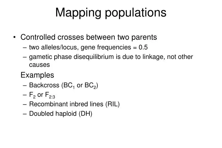
Mapping populations. Controlled crosses between two parents two alleles/locus, gene frequencies = 0.5 gametic phase disequilibrium is due to linkage, not other causes Examples Backcross (BC 1 or BC 2 ) F 2 or F 2:3 Recombinant inbred lines (RIL) Doubled haploid (DH).

E N D
Mapping populations • Controlled crosses between two parents • two alleles/locus, gene frequencies = 0.5 • gametic phase disequilibrium is due to linkage, not other causes Examples • Backcross (BC1 or BC2) • F2 or F2:3 • Recombinant inbred lines (RIL) • Doubled haploid (DH)
♀ ♂
Recombinant Inbred Lines (RILs) expected frequency
RILs R R R R
Doubled Haploids (DHs) expected frequency
DOUBLED HAPLOIDS R R R R R R R R R R
Expected Genotypic Frequencies for F2 Progeny when r = 0 or r = 0.5 Between Two Loci in Coupling (AB/ab) Configuration
Expected and Observed Genotypic FrequenciesCoupling (AB/ab) and Repulsion (Ab/aB) F2 Progeny • Co-dominant • Fully classified double hets. • Locus A = A and a • Locus B = B and b • r = recombination frequency between locus A and B
Expected and Observed Genotypic FrequenciesCoupling (AB/ab) F2 Progeny • Co-dominant • Unclassified double heterozygotes • Locus A = A and a • Locus B = B and b • r = recombination frequency between locus A and B
Expected and Observed Genotypic FrequenciesCoupling (AB/ab) and Repulsion (Ab/aB) F2 Progeny • Dominant • Locus A = A and a • Locus B = B and b • r = recombination frequency between locus A and B
Analysis • Single-locus analysis • Two-locus analysis • Detecting linkage and grouping • Ordering loci • Multi-point analysis
Mendelian Genetic Analysis Phenotypic and Genotypic Distributions • The expected segregation ratio of a gene is a function of the transmission probabilities • If a gene produces a discrete phenotypic distribution, then an intrinsic hypothesis can be formulated to test whether the gene produces a phenotypic distribution consistent with a expected segregation ratio of the gene • The heritability of a phenotypic trait that produces a Mendelian phenotypic distribution is ~1.0. Such traits are said to be fully penetrant • The heritability of a DNA marker is theoretically ~1.0; however, it is affected by genotyping errors
Mendelian Genetic Analysis Hypothesis Tests • The expected segregation ratio (null hypothesis) is specified on the basis of the observed phenotypic or genotypic distribution • One-way tests are performed to test for normal segregation of individual phenotypic or DNA markers • If the observed segregation ratio does not fit the expected segregation ratio, then the null hypothesis is rejected. • The expected segregation ratio is incorrect • Selection may have operated on the locus • The locus may not be fully penetrant • A Type I error has been committed
Mendelian Genetic Analysis Hypothesis Tests • Two-way tests are performed to test for independent assortment (null hypothesis - no linkage) between two phenotypic or DNA markers. • If two genes do not sort independently, then the null hypothesis is rejected • The two genes are linked (r < 0.50) • The expected segregation ratio is incorrect • A Type I error has been committed.
One-way or single-locus tests Goodness of fit statistics • C2statistics • Log likelihood ratio statistics • (G-statistics) Pr[C2 > 2df] = Pr[G > 2df] = i = ith genotype (or allele, or phenotype)
One-way or single-locus tests Two backcross populations (A and B) genotyped for a co-dominant marker (Brandt and Knapp 1993) Null hypothesis 1:1 ratio of aa to Aa i = ith genotype k = 2 genotypic classes Individual G-statistics for samples A and B Pr[GA > 2k-1] = Pr[14.8 > 21] = 0.0001 Pr[GB > 2k-1] = Pr[6.88 > 21] = 0.0086 Null hypothesis is rejected for both samples
One-way or single-locus tests Null hypothesis 1aa to 1Aa ratio for pooled samples Two backcross populations (A and B) genotyped for a co-dominant marker (Brandt and Knapp 1993) i = ith genotype j = jth sample k = genotypic classes p = No. of samples (populations) Pooled G-statistic across samples Pr[GP > 2k-1] = Pr[20.7 > 21] = 0.0000054 Null hypothesis is rejected
One-way or single-locus tests Two backcross populations (A and B) genotyped for a co-dominant marker (Brandt and Knapp 1993) Null hypothesis Samples A and B are homogenous i = ith genotype j = jth sample (population) k = genotypic classes p = No. of samples (populations) n = Total No. of observations The heterogeneity G-statistic is Pr[GH > 2(k-1)(p-1)] = Pr[0.94 > 21] = 0.33 (N.S.)
One-way or single-locus tests Relationship between G statistics Pr[GT > 2p(k-1)] = Pr[21.7 > 22] = 0.00002 k = genotypic classes p = No. of samples (populations)
One-way or single-locus tests F2 progeny of Ae. cylindrica genotyped for the SSR marker barc98. Null hypothesis 1:2:1 ratio of aa:Aa:AA i = ith genotype k = 3 genotypic classes Individual G-statistics for samples A and B Pr[G > 2k-1] = Pr[1.67 > 22] = 0.434 Null hypothesis is not rejected
Calculating probability values for Chi-square distributions SAS program data pv; Input x df; datalines; 3.75 2 ; data pvalue; set pv; pvalue = 1 – probchi (x, df); output; proc print; run; Output Obs x df pvalue 1 3.75 2 0.15335 Excel formula =CHIDIST(x , degrees_fredom) =CHIDIST(3.75 , 2) Output 0.15335