Download
1 / 46
460 likes | 616 Views
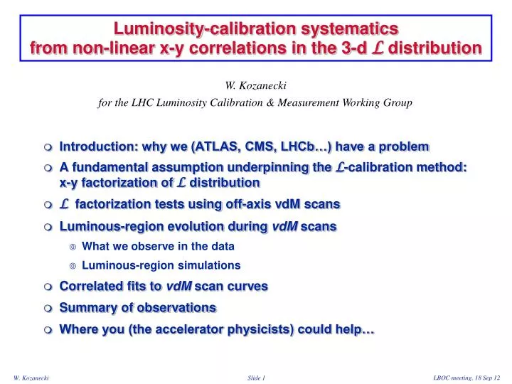
Luminosity -calibration systematics from non-linear x-y correlations in the 3-d L distribution. Introduction: why we (ATLAS, CMS, LHCb…) have a problem A fundamental assumption underpinning the L -calibration method: x-y factorization of L distribution

E N D
Luminosity-calibration systematics from non-linear x-y correlations in the 3-d L distribution • Introduction: why we (ATLAS, CMS, LHCb…) have a problem • A fundamental assumption underpinning the L-calibration method: x-y factorization of L distribution • L factorization tests using off-axis vdM scans • Luminous-region evolution during vdM scans • What we observe in the data • Luminous-region simulations • Correlated fits to vdM scan curves • Summary of observations • Where you (the accelerator physicists) could help… W. Kozanecki for the LHC Luminosity Calibration & Measurement Working Group
Introduction: a problem? but…where? why? • The vdM-based calibrations for 2011 reached a level of precision unprecedented at hadron colliders (except for the ISR) • DL / L = 1 .8 % [May’11 vdM scans, ATLAS-CONF-2012-080, ICHEP 2012] • LHCb/CMS: comparable/slightly larger uncertainties (LumiDays ‘12) • Two very challenging issues surfaced in 2012 • the ‘rising visible cross-section’ problem (April + July 2012 vdM scans) • breakdown of x-y factorization in the 3-d L distribution (Jul ’12 scans) ~ 2.5 % Rising svis also observed by CMS Jul’12 vdM scans Apr’12 vdM scans
A fundamental assumption: x-y factorization of L (Dx, Dy) • A key assumption of the vdM scan method as currently applied is that the luminosity factorizes in x & y: • This is equivalent to assuming that the shape of the scan curve during an x (y) scan is independent of the separation Dy (Dx) in the orthogonal plane • if this is the case, the combination of 1 x-scan and 1 y-scan is sufficient to characterize the entire distribution L (Dx, Dy) • if this is violated at a “significant” level, the vdM formalism can be generalized to 2 dimensions by performing a grid scan (impractical!) • Although linear x-y coupling does violate this assumption, the induced bias is typically very small (DL/L ~ 0.1%) with present LHC optics (small x-y coupling coeff., ex ~ ey, b*x ~ b*y)
The “beam size” and its avatars The assumption that the luminosity distribution contains no x-y correlations, can be tested by performing off-axis vdM scans (x-scan with y offset, y- scan with x offset)
Off-axis scans in F 2856 (ATLAS Jul ‘ 12 vdM scan) F 2856 ~1/50 ~1/30 Scan VIII: x , y Scan IX: x w/ y offset, y w/ x-offset Partial beam separation for ATLAS offset scans: 344 (369) m for scan VII (IX)(adjusted to correspond to Dx,y ~ 2.6 - 2.8 Sx and to an integer # steps)
On-/off-axis scans in ATLAS & CMS: Sx comparison (BCID average) • Note that CMS used a significantly smaller partial separation (1S) in off-axis scans than ATLAS did (2.4-2.8 S) • Effect also seen in LHCb (~ 4% on S, for D ~ 1.4 S ) Scans VII, IX (offset) 4 % 15 % 9 % Scans VI, VIII (centered)
Luminous-region evolution in Jul ’12 (BCID-av): widths, x-scans Centered scans 10 % Offset scan y-width during x-scan depends on y offset! Centered scans Offset scan 60 %
Luminous-region evolution in Jul ’12 (BCID-av): widths, y-scans Centered scans x-width during y-scan depends on x offset! Convincing evidence for non-linear correlations … so are the earlier (7 TeV) calibrations valid ? Offset scan and how large is the ultimate uncertainty on the 8 TeV calibrations? y-width during y-scan depends on x offset!
Luminous-centroid evolution during vdM scans: Oct’ 10 vs. May ‘11 May 2011 Oct 2010 x-displacement Non-gaussian tails! sx/sy sx,1/sx,2 y-scans y-scans x-scans x-scans y-displacement Non-gaussian tails! sy,1/sy,2 sy/sx z-displacement ay,z ax,z
Luminous-centroid evolution during vdM scans: Oct’ 10 vs. May ‘11 May 2011 Oct 2010 x-displacement Non-gaussian tails! sx/sy sx,1/sx,2 y-scans y-scans x-scans x-scans y-displacement Non-gaussian tails! sy,1/sy,2 sy/sx Note that for strictly gaussian beams (even if unequal in x v.s y and B1 vs. B2, and even with linear x-y coupling), the transverse luminous sizes are independent of the beam separation during vdM scans. z-displacement ay,z ax,z
Luminous-region simulations • Aim: try & reproduce beam spot displacement & changes in luminous widths observed during vdM scans • Procedure • Use a simple simulation written in Mathematica to gain an intuition for the required beam parameters • Assumptions • double-Gaussian beam profiles • ignore crossing angles (for now) • Quantitative interpretation of luminous-region parameters • real data: max. likelihood fit of resolution-corrected, 3-d single-gaussian to reconstructed-vertex distribution • this simulation (so far) • luminous centroid = mean • luminous width = RMS L x y
Luminous-region simulations: examples sLx (mm) Dx (mm)
Luminous-region evolution: model 2b, x-scan, y-centered (May’11 vdM) x-centroid y-centroid <x>L(mm) <y>L(mm) Dx (mm) Dx (mm) x-width y-width sxL(mm) syL(mm) Dx (mm) Dx (mm)
Luminous-region evolution: model 2b, x-scan, y offset (May’11 vdM) x-centroid y-centroid <x>L(mm) <y>L(mm) Dx (mm) Dx (mm) y-width x-width sxL(mm) syL(mm) Dx (mm) Dx (mm)
A complementary approach: correlated fits to vdM scan curves • To estimate (roughly) the magnitude of a potential NLC-induced bias, ATLAS routinely compared the visible cross-sections (i.e. the L calibration scales) obtained by fitting the x- & y- vdM-scan curves using either • an uncorrelated model (= baseline): g+g (can simplify to g, or to g+p0) • a correlated double-gaussian model (naïve & by no means unique) that reduces to the uncorrelated model at Dx = Dy = 0 (but with fx = fy) • Observed impact on visible cross-sections at √s = 7 TeV (ATLAS) • Dsvis / svis ~ 3%, 2%, 0.9%, 0.5 % for Apr ’10, May ’10, Oct ’10, May ’11 • The more single-gaussian the scan curves, the smaller the potential bias (a property of this model – but probably not a general property?) • As the effect looked small for the two main 7 TeV scan sessions, and for lack of manpower, we didn’t look much further until … L(x, y) L(x, y)
Correlated fits to vdM scan curves: Mar ’11 scans (2.76 TeV pp) LUCID_OR
Correlated fits to vdM scan curves: Mar ’11 scans (2.76 TeV pp) LUCID_OR
Correlated fits to vdM scan curves: Apr ’12 scans (8 TeV pp)
Correlated fits to vdM scan curves: Apr ’12 scans (8 TeV pp) • Notes • the true bias may be larger than the difference between uncorrelated & correlated fits (coupling model dependence!) • there may be other coupling models which also yield a stable central value, but significantly different from the present one. To be studied. • The same analysis is being applied to May’11 & Jul’12 vdM scans
Summary (1) • Assumption that L distribution factorizable in x, y appears violated • as manifested by • differences in fitted Sx,y values in centered & off-axis vdM scans • differences in luminous-width evolution during centered & off-axis scans • sensitivity of the visible cross-sections to an x-y correlated fit model • to a different degree in different scan sessions • in a manner that is only partially correlated with the amplitude of non-gaussian tails in the x- and/or y- luminosity-scan curves • Compelling evidence that this is caused by the beams themselves • never considered at other colliders • urgent (and still ongoing) review of the potential impact of NLC’s in the systematic uncertainty affecting the ATLAS vdM calibrations of May’11 (7 TeV) and March ‘11 (2.76 TeV) • evaluation of • the impact on the precision of the absolute L scale in 2012 (all 4 expts!) • the potential need for an additional vdM scan in 2012. Prerequisites: • understand how large the L uncertainty may be without it • convincing arguments that we can do better – and how ( LBOC)
Summary (2) • An analytical framework is now in place for the linear analysis of the luminous-region evolution during vdM scans. • Assumptions • each beam = single-gaussian • x-y [can be] linearly correlated • Deviations from this linear model (observed at large beam separation) clear signature for the non-gaussian character of the L(x, y,z) distribution (info independent from / complementary to L-scan curves) • Simulations have started for the analysis of luminous-region evolution during scans, under more general assumptions: • each beam = double gaussian w/ common mean • the 4 gaussians (B1/B2, x/y) [can] have different x-y correlations These simulations • allow a 3-d visualization of the L(x,y) distribution, making it possible to develop a physical intuition for the complex structures that result from some beam-parameter configurations • not (yet) successful in setting upper limit on the May’11 uncertainties
Summary (3) • Allowing for non-linear x-y correlations (NLC) in vdM fits improves the scan-to-scan svis consistency (one specific, naïve model tried!) in the March ‘11 and Apr’12 vdM scans. To do: May ’11, Jul ’12 • may explain large scan-to-scan inconsistencies in Apr & Jul vdM calibs • but NLC-induced bias may be larger than the observed inconsistencies • Next steps • ATLAS ‘to-do’ list • Correlated vdM fit May ‘11 & Jul ‘12 scans; more coupling models! • Luminous-region simulation of Jul’12 scans (stronger signals -> easier?) • The present characterization of the (measured or simulated) L(x,y) distribution is oversimplified (mean+RMS, or 1G fit); a more sophisticated parameterization/fit of the beam spot is needed • Combined fit to the luminosity-scan and luminous-region data (a significant investment!) [as suggested in 2011 by A. Messina & G. Piacquadio] • CMS, LHCb, ALICE now in the loop, starting to • perform correlated vdM fits to available 2011 & 2012 scans • compare luminous-region evolution in centered & offset scans • LHCb • provide both 1-d and 2-d (x-y) single-beam profiles (SMOG, July’12 scans)
Where you (accelerator physicists) could help… • The more gaussian the beams, the smaller the potentially harmful correlations. The vdM scan curves were • almost perfectly single Gaussians in May 2011 (F 1783) • imperatively require g+g (or more complex) fits in other scan sessions • wire scans in 2012 (F 2520, 2855, 2856) highly non-gaussian; F1783 ?? • limited dynamic range (< x 10) • projections only • what other techniques can be used to characterize x-y beam shapes? • what was special about May 2011 ? • what can be done to make the beams more gaussian (during vdM scans)? • did the improvements on injected einv during Aug 2012 make the beams more gaussian? • Could be tested by end-of-fill scans
V. Kain Wire scans during Jul ’12 ATLAS/CMS scans (F 2856)
V. Kain Wire scans during Jul ’12 ATLAS/CMS scans (F 2856) • Observations • 2nd-gaussian more prominent in the vertical (in this fill only – or is this typical?) • large 2nd gaussian in both H & V at injection (previous fill) • dynamic range < factor of 10; L sensitive way beyond this)
Where you (accelerator physicists) could help… • The more gaussian the beams, the smaller the potentially harmful correlations. The vdM scan curves were • almost perfectly single Gaussians in May 2011 (F 1783) • imperatively require g+g (or more complex) fits in other scan sessions • wire scans in 2012 (F 2520, 2855, 2856) highly non-gaussian; F1783 ?? • limited dynamic range (< x 10) • projections only • what other techniques can be used to characterize x-y beam shapes? • what was special about May 2011 ? • what can be done to make the beams more gaussian (during vdM scans)? • did the improvements on injected einv during Aug 2012 make the beams more gaussian? • Could be tested by end-of-fill scans • What could be the source(s) of the observed non-factorization? • beam-beam probably excluded (WH @ LumiDays: dynamic b ~ 0.5%) • large bunch-by-bunch differences => caused (only partly?) by injectors • octupoles? (stronger now than in May’11 ?) • impedance? skew quad term?
Where you (accelerator physicists) could help… (2) • Related observations (may or may not be relevant to today’s problem) • “shape” of luminosity distribution region evolves during fill • does not just ‘scale’ with e growth • fraction of wider gaussian increases • relative centers of the wide & narrow gaussians movefurther apart • strong left-right asymmetry in scan curves (also seen by CMS) • cannot be accomodated by linear optics (betatron oscillations) • can be tested by scanning in one direction and then immediately in the other
Apr’12 scans are labelled scans I-III Overview of July ‘12 scan program at IP 1 & 5 F 2855 DSC: B1X, B2X, B1Y BI checks VII: x –y w/ offset VI: x -y V: x -y IV: x -y F 2856 IX: x –y w/ offset DSC: B2Y VIII: x -y
Systematic uncertainties on absolute L at 7 TeV • The vdM-based calibrations for 2011 reached a level of precision unprecedented at hadron colliders (except for the ISR) • ATLAS example (May’11 vdM scans, ATLAS-CONF-2012-080) • LHCb/CMS: comparable/slightly larger uncertainties (LumiDays ‘12) vdM-calibration uncertainties Total L uncertainty BUT… are these uncertainties RIGHT?
On- and off-axis scans in ATLAS (Jul ‘ 12 vdM): Sy comparison
Online fits to BCID-blind scan curves: Sy (g+p0[B]) Note that CMS used a significantly smaller partial separation in off-axis scans than ATLAS Effect also seen in LHCb Scans VII, IX (offset) Scans VI, VIII (centered)
Luminous-centroid evolution during May ‘11 vdM (centered) scans These plots show the position of the luminous centroid during the first set of x and y scans in May 2011. A linear fit, based on an analytical description of x-y coupled, single-gaussian beams,has been made to the central scan data (separation |h| < 0.05 mm). The linear fit gives the gradient of the movement, and corresponds to the extraction of the observables in Table 1. The diagonal plots (a), (d) clearly indicate the presence of non-gaussian tails. y-scan Hor. displacement x-scan Hor. displacement y-scan Vert. displacement x-scan Vert. displacement
Luminous-centroid evolution during vdM scans: interpretation(assuming each beam is Gaussian) The plots on the preceding page show the position of the luminous centroid during the first set of x and y scans in Oct 2010 &May 2011. A linear fit, based on an analytical description of x-y coupled, single-gaussian beams, has been made to the central scan data (separation |h| < 0.05 mm). The linear fit gives the gradient of the movement, and corresponds to the extraction of the observables in the Table below (Linear) Note that for strictly gaussian beams (even if unequal in x v.s y and B1 vs. B2, and even with linear x-y coupling), the transverse luminous sizes are independent of the beam separation during vdM scans.
Luminous-region evolution in Jul ’12 (BCID-av): centroids, x-scans Centered scans Evidence for non-gausssian tails! Offset scan
Luminous-region evolution in Jul ’12 (BCID-av): centroids, y-scans Centered scans Offset scan Clear evidence for non-gausssian tails!
Luminous-region simulations (2) sLx (mm) Dx (mm)
Luminous-region simulations (4) sLy(mm) Dx (mm)
Modelling of luminous-region evolution during May’11 vdM scans • Goal • determine a set of beam parameters (each beam = double gaussian) that reproduce both • the beam-separation dependence of luminous-region parameters (centroid position, luminous width) • the luminosity variation (i.e. Sx,y ) during the May ‘11 vdM scans (both centered and offset scans) • for this parameter set, compute the fractional difference between • the luminosity computed from the values of Sx,y as fitted to the simulated centered scans (as is done with real data) • the ‘true’ luminosity, obtained by integrating the 2-d or 3-d L distribution • Procedure • estimate first-order parameters (core gaussians) from the results of the linear analysis • adjust (by hand, guided by physical intuition) the other parameters to reproduce the separation-dependence of the beamspot parameters, respecting (to some degree) the constraints from measured Sx,y values • iterate…
Modelling of May ’11 vdM scans: parameter sets Model 1 Model 2b • Note that • the coupling terms of the core gaussians (ka) are either 0 or very small • the coupling terms of the tail gaussians (kb) are both 0 • so that in practice, both of these luminosity models are (almost) totally uncorrelated. • Whether this is • serendipitous, and reflects the limitations inherent to a manual procedure • imposed by the data themselves, • remains to be determined. Xing angle = 240 mrad Xing angle neglected
Luminous-region evolution: model 2b, y-scan, x-centered (May’11 vdM) x-centroid y-centroid <x>L(mm) <y>L(mm) Dy (mm) Dy (mm) x-width y-width sxL(mm) syL(mm) ay,z Dy (mm) Dy (mm)
Luminous-region evolution: model 2b, y-scan, x offset (May’11 vdM) x-centroid y-centroid <x>L(mm) <y>L(mm) Dy (mm) Dy (mm) x-width y-width sxL(mm) syL(mm) Dy (mm) Dy (mm)
vdM parameters: modelledvs.measured • Observations • Large (several %) differences between both models and the data, in terms of S and therefore of predicted Lsp • For centered scans, model 2b typically reproduces the measured S’s better. However the ~ 6% difference between Sx and Sy, expected from the crossing angle, is not reproduced. • For offset scans, model 1 reproduces better the offset/centered S ratio • Both models predict a small (0.2 -0.5%) bias on reference L – but this doesn’t (yet?) mean much in view of the large inconsistencies in (a) predicted S and (b) separation-dependence of luminous-region variables
Summary: May’11 studies • This simulation tool has been applied to a (manual) exploration of the beam-parameter space in an attempt to model the May’11 vdM beamspot data, both centered and offset. Main conclusions: • each BCID behaves differently, so at least part of the non-linear correlations arise in the LHC injector chain • the simulation can reproduce the centered scans reasonably well, but did not succeed (so far) to reproduce the offset scans simultaneously • whether the crossing-angle effects are correctly modelled needs to be checked • because the vertexing-resolution effects are large, constraining the input beam parameters with the measured S’s is essential. This has not been achieved yet – at least at the required level of precision
Correlated fits to vdM scan curves: Mar ’11 scans (2.76 TeV pp)
(Un)correlated fits to vdM scan curves: May ’11 & Jul ’12 • Uncorrelated fits • Correlated fits: to be done! Jul ‘12 (8 TeV, 4 centered scans) May ’11 (7 TeV, 2 centered scans) ~ 2.5 % ~ 0.5 % Note that the true bias may be larger than the scan-to-scan inconsistency