Download
1 / 11
110 likes | 114 Views
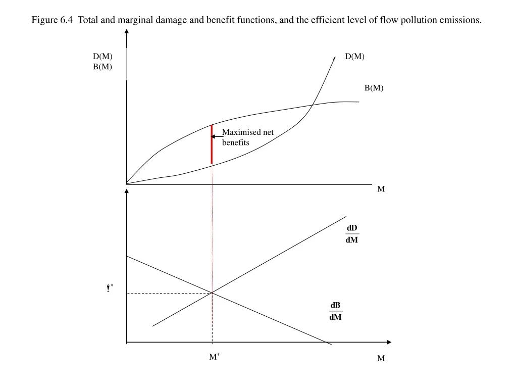
This figure shows the total and marginal damage and benefit functions, as well as the economically efficient level of flow pollution emissions. It also demonstrates how setting targets based on health criteria and spatial differentiation can help achieve efficient pollution control. The figure further explores the concept of threshold effects and irreversibilities in pollution management. Lastly, it illustrates non-convex damage functions arising from pollution saturation and concentration-dependent effects.

E N D
Figure 6.4 Total and marginal damage and benefit functions, and the efficient level of flow pollution emissions. D(M) B(M) D(M) B(M) Maximised net benefits M * M* M
Figure 6.5 The economically efficient level of pollution minimises the sum of abatement and damage costs. £ Marginal damage C3 * C1 Marginal abatement cost C2 M Quantity of pollution emission per period 0 MA M*
Figure 6.6 Setting targets according to an absolute health criterion. Marginal health damage t* MC MH Emissions, M
Figure 6.7 A ‘modified efficiency’ based health standard. Marginal health damage tH* MC MH* Emissions, M
Figure 6.8 A spatially differentiated air shed. R1 R2 S1 S2 R4 R3
Figure 6.9 Efficient steady-state emission level for an imperfectly persistent stock pollutant. Two cases: {r = 0 and > 0} and {r > 0 and > 0}. ** * M** M M*
Figure 6.10 Threshold effects and irreversibilities. Figure 6.10a A threshold effect in the decay rate/pollution stock relationship. A
Figure 6.10(b) An irreversibility combined with a threshold effect. A
f(x) a b • • x Figure 6.11 A strictly convex function
D D MS M MD = dD/dM MD MS M Figure 6.12 A non-convex damage function arising from pollution reaching a saturation point.
Figure 6.14 A non-convex damage function arising from pollutants harmful at low concentrations but beneficial at higher concentrations. £ Marginal benefit Marginal damage a b C M Quantity of pollution emission per period 0 M1 M2 M3 M4