Linear Operations Using Masks

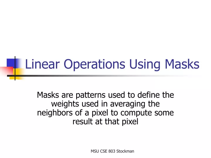
1. Linear Operations Using Masks Masks are patterns used to define the weights used in averaging the neighbors of a pixel to compute some result at that pixel MSU CSE 803 Stockman

2. Expressing linear operations on neighborhoods MSU CSE 803 Stockman

3. Images as functions MSU CSE 803 Stockman

4. Neighborhood operations • Average neighborhood to remove noise or high frequency patterns • Detect boundaries at points of contrast using gradient computation • Can use median filtering to smooth while keeping boundaries sharp MSU CSE 803 Stockman

5. Image processing examples Histogram equalization; gamma correction; median filtering MSU CSE 803 Stockman

6. Histogram equalization Left image does not use all available gray levels. Image is recoded so that all gray levels are used and such that each gray level occurs in roughly the same number of pixels of the recoded image. (See algorithm in text, xv.) MSU CSE 803 Stockman

7. Histogram equalization can darken a bright image, perhaps improving contrast MSU CSE 803 Stockman

8. Can define mapping of input gray level to output level (xv) Gamma correction: boost all gray levels Boost low levels and reduce high MSU CSE 803 Stockman

9. Smoothing an image by averaging neighbors (boxcar) MSU CSE 803 Stockman

10. Output pixel is the dot product of the input neighborhood and the mask MSU CSE 803 Stockman

11. Properties of smoothing masks MSU CSE 803 Stockman

12. Types of ideal edges (in 1D) These types are also present in 2D and 3D images and are complicated by orientation variations. MSU CSE 803 Stockman

13. Boxcar smoothing filter example So, reducing noise will also degrade the signal. MSU CSE 803 Stockman

14. Linear smoothing smoothes noise and blurs signal Blur: step is now ramp Input image Row after 5x5 mean filter MSU CSE 803 Stockman

15. Gaussian smoothing MSU CSE 803 Stockman

16. Median filter replaces center with neighborhood median, not mean Median filter smoothes signal and preserves sharp boundary Mean filtering smoothes signal and ramps the boundary Noisy row of checkers image MSU CSE 803 Stockman

17. Median filter is not linear • Algorithm requires comparisons and is more expensive than using mask • Can sort all NxN pixel values and pick middle • Do not need totally sorted data: O(N) algorithm exists MSU CSE 803 Stockman

18. Scratches removed by using a median filter Thin artifact removed, sharp boundaries preserved. MSU CSE 803 Stockman

19. Finding boundary pixels Computing derivatives or gradients to locate region change. MSU CSE 803 Stockman

20. 2 rows of intensity vs difference MSU CSE 803 Stockman

21. Differencing used to estimate 1st and 2nd derivatives Masks represent the first and 2nd differences First differences 2nd differences MSU CSE 803 Stockman

22. Step edges X mask [-1, 0, +1] Step edge is detected well, but edge location imprecise. MSU CSE 803 Stockman

23. Ramp and impulse X mask [-1, 0, +1] Ramp edge now yields a broad weak response. Impulse response is a “whip”, first up and then down. MSU CSE 803 Stockman

24. 2nd derivative using mask [-1, 2, -1] Response is zero on constant region and a “double whip” amplifies and locates the step edge. MSU CSE 803 Stockman

25. 2nd derivative using mask [-1, 2, -1] Weak response brackets the ramp edge. Bright impulse yields a double whip with gain of 3X original contrast. MSU CSE 803 Stockman

26. Estimating 2D image gradient MSU CSE 803 Stockman

27. Gradient from 3x3 neighborhood Estimate both magnitude and direction of the edge. MSU CSE 803 Stockman

28. Prewitt versus Sobel masks Sobel mask uses weights of 1,2,1 and -1,-2,-1 in order to give more weight to center estimate. The scaling factor is thus 1/8 and not 1/6. MSU CSE 803 Stockman

29. Computational short cuts MSU CSE 803 Stockman

30. Alternative masks for gradient MSU CSE 803 Stockman

31. Computational shortcuts • Use MAX operation on 1D row and column derivatives. • Use OR operation on thresholded row and column derivatives. MSU CSE 803 Stockman

32. 2 rows of intensity vs difference MSU CSE 803 Stockman

33. Caption for Prewitt image MSU CSE 803 Stockman

34. Properties of derivative masks MSU CSE 803 Stockman

35. Next set of related slides Interpret the properties of masks using the theory of vectors and dot products. MSU CSE 803 Stockman