Download
1 / 49
490 likes | 585 Views
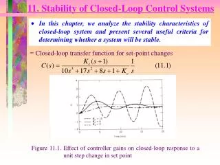
Plant-wide Monitoring of Processes Under Closed-loop Control. Sergio Valle-Cervantes Dr. S. J. Qin: Advisor Chemical Engineering Department University of Texas at Austin. Outline. Introduction Objective Selection of the number of principal components

E N D
Plant-wide Monitoring of Processes Under Closed-loop Control Sergio Valle-Cervantes Dr. S. J. Qin: Advisor Chemical Engineering Department University of Texas at Austin
Outline • Introduction • Objective • Selection of the number of principal components • Extracting fault subspaces for fault identification of a polyester film process • Multi-block analysis with application to decentralized process monitoring • Extension to the MBPCA analysis with fault directions and wavelets. • Conclusions
Introduction • Faults in industry • Among others, bad products, insecure conditions, damage to the equipment. • In summary, lost of millions of dollars just because faults are not detected and identified on time • Just in the U.S.A. petrochemical industries an annual loss of $20 billions in 1995 has been estimated because of poor monitoring and control of such abnormal situations • Actually: • Chemical process highly automated • The quantity of data captured by the information system is amazing
Introduction • What can we do? • Use this huge quantity of data to monitoring, control and optimize the process • Actually, the modern computer systems are able to analyze that information, something in the past was not possible • Therefore, efficient methods to on time fault detection and identification has been one of the main targets in industry to the afore mentioned.
Objectives • Obtain novel methods for process monitoring, fault detection and identification using PCA. • Use PCA and PLS models to identify the main factors that affect the process • Determine the number of principal factors necessary to describe the process but not noise. • Provide industry with new ways to improve the process operations. • Develop new monitoring tools to increase process efficiency, thereby reducing costs and off-specification products. • Develop plant-wide monitoring strategy under closed-loop control, including sensor fault detection, loop performance monitoring and disturbance detection.
Selection of the number of PC’s • One of the main difficulties in PCA: selection of the # of PC’s. • Most of the methods use monotonically increasing or decreasing indices. • The decision to choose the # of PC’s is very subjective. • A method based on the variance of the reconstruction error to select the # of PC’s. • The method demonstrates a minimum over the # of PC’s. • Ten other methods are compared with the proposed method. • Data sets: incinerator, boiler, and a batch reactor simulation.
Fewer or more PC’s? • Key issue in PCA # of PC’s • If fewer PC’s than required: • A poor model will be obtained • An incomplete representation of the process • If more PC’s than necessary: • The model will be overparameterized • Noise will be included
Methods to choose the # of PC’s • Two approaches to obtain the # of PCs: • Knowledge of the measurement error • Use of statistical and empirical methods • Akaike information criterion (AIC) • Minimum description length (MDL) • Imbedded error function (IEF) • Cumulative percent variance (CPV) • Scree test on residual percent variance (RPV) • Average eigenvalue (AE) • Parallel analysis (PA) • Autocorrelation (AC) • Cross validation based in Rratio • Variance of the reconstruction error (VRE)
AIC and MDL: popular in signal processing. IEF in factor analysis. Common attributes: Work only with covariance-based PCA Variance of measurement noise in each variable are assumed to be identical A minimum over the number of PC’s. AIC, MDL, and IEF
CPV: measure of the percent variance captured by the first l PCs. Scree test on RPV: the method looks for a “knee” point in the RPV plotted against the number of PCs. AE: accepts all eigenvalues above the average eigenvalue and rejects those below the average. PA: two models, original and uncorrelated data matrix. All the values above the intersection represent the process information and the values under the intersection are considered noise. Selection Criteria in Chemometrics
Autocorrelation: use an autocorrelation function to separate the nosy eigenvectors from the smooth ones. Cross validation based on the R ratio: R < 1 the new component improve the prediction, then the calculation proceeds. R > 1 the new component does not improve the prediction then should be deleted. Cross validation based on PRESS: Use PRESS alone to determine the number of PCs. A minimum in PRESS(l) corresponds to the best number of PCs to choose. Selection Criteria in Chemometrics
Based on the best reconstruction of the variables VRE index has a minimum, corresponding to the best reconstruction VRE is decomposed in two subspaces: The portion in PCS has a tendency to increase with the number of PC’s. The portion in the RS has a tendency to decrease. Result: a minimum in VRE. Variance of the Reconstruction Error
Examples: Batch Reactor • Simulated batch reactor • Isothermal batch reactor • 4 first order reactions • 2% of noise • 200 samples, 5 variables • Boiler • 630 samples, 7 variables • T, P, F, and C. • Incinerator • 900 samples, 20 variables. • T, P, F, and C.
Summary • Most of the methods have monotonically decreasing or increasing indices • The IEF, AC, AIC, and MDL worked well with the simulated example, but they failed with the real data. • The most reliable methods are: CPV, AE, PA, PRESS, and VRE. • Considering the effectiveness, reliability, and objectiveness, the PRESS method, and correlation based VRE method are superior to the others. • VRE is preferred to the PRESS method in the consistency of the estimate, computational cost, and ability to include a particular disturbance or fault direction in the selection.
Extracting Fault Subspaces for Fault Identification • As chemical processes becomes more complex: • Tightly control the process • Detect disturbances before they affect the process quality • Monitoring and diagnosis of chemical processes: • Asses process performance • Improve process efficiency • Improve product quality • More sensors > more data. • How to analyze the data to obtain the best process knowledge
Extracting Fault Subspaces for Fault Identification • Extracting the information is not trivial • Extremely important for chemical processes: • The analysis of sensor conditions • Process performance • Fault detection and identification are essential for a good monitoring system • Statistical process control • Based on control charts for certain quality variables • Multivariate statistical process control • Model process correlation, detect and classify faults, control product quality with long time delays, monitoring dynamic processes, and detect and identify upsets in multiple sensors.
Extracting Fault Subspaces for Fault Identification • Two indices used in PCA or PLS based monitoring: • Hotelling’s statistics T2: gives a measure of the variation within the PCA model. • Squared prediction error (SPE) of the residuals: indicates how much each sample deviates from the PCA model. • Often insufficient to identify the cause of the upsets. Then to identify the cause of the upsets: • Contribution plots • Sensor validity index
New Approach • To extract process fault subspaces from historical process faults using SVD. • Historical process data are first analyzed using PCA to isolate between normal and abnormal operations. • Process knowledge, operational and maintenance records are incorporated to assist the isolation of abnormal operation periods. • The abnormal operation data are used to extract the fault subspaces. • The extracted fault subspaces are used to reconstruct new abnormal data that are detected by the fault detection step. • If the new faulty data can be reconstructed by one of the extracted fault subspaces, fault identification is completed for the new faulty data. • Otherwise, the new faulty data are from a different type of fault that has not been recorded in the historical data. • A new fault subspace is then extracted from the data and is added to the fault data base for future fault identification.
The purpose of fault detection and identification is to improve the safety and reliability of the automated system PCA Detection indices: SPE Hotelling’s T2 Detection and Identification of Process Faults
Monitoring and Diagnosis Based on SPE Monitoring and Diagnosis Based on T2 Contribution Plots
Different grades of products are processed in the same equipment. A typical fault: sudden oscillation of some temperature loops which swings in 10 degrees, then stop after a while. Hundred of sensors used in the process, including temperature, thickness, tension, etc., with a gauge. Grade changes for different products are frequent, approximately once a day. Changes in set points are made more frequently, and if it is needed the operators change the set points manually. Currently: SPE always exceeds limits; contribution plots indicate multiple suspects and no limits; multiple grades with only one model clusters for different grades. Polyester Film Process
308 variables Process variables Set points Output variables Monitoring variables Process and monitoring variables were used in this analysis, 103 variables. Four clusters Red cluster: normal Blue, green, and black clusters: faulty. Data Analysis: clusters
Determining the number of PC’s. Four methods Average eigenvalue Parallel analysis Cumulative percent variance Variance of the reconstruction error. Fifteen PC’s were used to build the model. Data Analysis: PCs
The variables that are contributing to the out of control situation in this window of 250 samples are, mainly variable 28 and in a minor proportion variables 25 and 32 In particular for sample 71: Highest contribution: variable 28 Smaller contribution: variables 25, 32, and 93 Data Analysis: Contribution Plots
The fault directions are modeled from abnormal data. These directions are used to identify the true type of faults. Subplot(5,2,1) Highest direction variable 28 Subplot(5,2,2) Highest direction variable 25 Subplot(5,2,3) 32, 30, 29, 28, and 25 Subplot(5,2,4) 34 and 40 Fault Direction Extraction
The fault directions are extracted from the faulty SPE until it is under the limit defined by the PCA model. Nine fault directions are necessary to deflate the SPE under the threshold. Observe how the first peek in the original SPE is deflated immediately after the first direction is extracted (second plot). And the residual peek in the second plot is deflated after subtracting the next direction (third plot). SPE deflation
First subplot: The SPE for a window of 125 samples in the testing data. Second subplot: The reconstructed SPE on the testing data after extracting the fault directions. The fault is partially identified. Third subplot: The fault identification index shows a tendency to increase after sample 80, that is because no fault was identified there. The fault has been identified in the first part, between sample 20 and 80. Fault Identification
Summary • With the extraction of fault directions from historical data, it is possible to identify process faults for the out-of-control situation. • These directions are “signatures” that characterize certain types of faults. • It is viable to use them to identify similar faults in the future. • This technique requires only historical faulty data to model the fault directions and normal data to build a PCA process model. • In the case that a new type of faults is identified, the new fault subspace is extracted and stored for future fault identification. • In this way the number of fault subspaces can grow as more faults are encountered.
Multi-block Analysis • Large processes • Hundred of variables (difficult to detect and identify faults) • Divide the plant in sections or blocks • Using multi-block algorithms localize the faulty section or block. • Basic idea: divide the descriptor variable (X) into several blocks in the PCA case, to obtain local information (block scores) and global information (super scores) simultaneously from data. • Use the regular PCA to calculate block scores and loadings based on the scores. • The use of multi-block analysis methods for process monitoring and diagnosis can be directly obtained from regrouping contributions of regular PCA model.
Regular PCA algorithm Regular PLS algorithm Regular Algorithms
CPCA algorithm based on PCA scores MBPCA algorithm based on PCA loadings CPCA and MBPCA
Based on SPE: Based on T2 Monitoring and Diagnosis No fault No fault
A standard PCA model is applied to all the variables. Identification of the out-of-control situation variables is difficult. SPE and T^2 do not agree in all the variables. Contribution plots does not have a confidence limit. Standard MSPC monitoring
Process data is divided in 7 blocks. Faulty block is located applying decentralized monitoring. Block 2 is where the main fault is located. SPE for each block
In block 2 is identified the largest contribution. Variables 28 and 25 are mainly responsible for the out-of-control situation using contribution plots. Identification of the variables is clearer with CPCA than with standard MSPC monitoring. Identification of Faulty Blocks Using SPE
T2 also shows that the main fault is located in the second block. Again variables 28 and 25 are identified. The decentralized monitoring approach gives a much clearer indication of the faulty variables. Identification of Faulty Blocks Using T2
The SPE index is shown for all blocks along samples of data. Any significant departure from the horizontal plane is an indication of a fault. Block SPE Index
Summary • The use of multi-block PCA and PLS for decentralized monitoring and diagnosis is derived in terms of regular PCA and PLS scores and residuals. • The decentralized monitoring method based on proper variable blocking is successfully applied to an industrial polyester film process. • Using the subspace extraction method and decentralized monitoring PCA method, it is shown that the identification of the fault is clearer than using a whole PCA model. • What we need is only good faulty data to extract the “signature” of the fault. • Future task is use recursive PCA, or recursive PLS for adaptive decentralized monitoring. • Develop fault identification index to uniquely identify the root cause of a fault instead of contribution plots. • Integrate multi-scale monitoring approach in the decentralized monitoring approach for partitioning the data, to provide flexible partition and interpretation of information contained in the process data.
Multi-Block PCA and FII • Instead of extracting the fault directions using one PCA model for the whole plant, now extract the directions only in the faulty block. • The information required to identify a new fault is less than using the whole PCA model.
Fault directions are extracted from the SPE until it is under the limit defined by Three fault directions are necessary to deflate the SPE under the threshold. In the whole PCA model it was necessary to extract 9 directions. Fault Direction Extraction: Block 2
Directions that will be used to identify the true faults in a new data set. Clearly it is shown that variables 19 and 16 are the variables mainly responsible for the out-of-control situation. The projections here are more clear that using the whole PCA model. Fault Directions
First subplot The SPE for 125 samples for the testing data is shown. Second subplot The reconstructed SPE on the testing data after extracting the fault directions, identifies the fault. Third subplot The fault identification index value goes to zero from sample 20 to sample 90, then the fault is identified. After sample 100 a new fault arrives to the system Fault Identification
Conclusions and Future Work • The merging of MBPCA and the directions extraction has bettered the identification of the fault. • Less quantity of information to needed to identify new faults. • Integrate in this new approach the multi-scale monitoring approach for partitioning the data, to provide flexible partition and interpretation of information contained in the process data. • Use dynamic PCA modeling to extract the full process model and capture the true characteristics of the process.
Related Publications • S. Valle, W. Li, and S. J. Qin, “Selection of the Number of Principal Components: the Variance of the Reconstruction Error Criterion with a Comparison to Other Methods”. Ind. Eng. Chem. Res., 38, 4389-4401 (1999) • W. Li, H. Yue, S. Valle, and S. J. Qin, “Recursive PCA for Adaptive Process Monitoring”, J. of Process Control., 10 (5),471-486 (2000) • S. Valle,S. J. Qin, and M. Piovoso, “Extracting Fault Subspaces for Fault Identification of a Polyester Film Process”. Submitted to ACC-2001 • S. J. Qin, S. Valle, and M. Piovoso, “On Unifying Multi-block Analysis with Application to Decentralized Process Monitoring”. Accepted by J. Chemometrics
Acknowledgements • National Science Foundation (CTS-9814340) • Texas Higher Education Coordinating Board • DuPont through a DuPont Young Professor Grant • Consejo Nacional de Ciencia y Tecnología (CONACyT) • Instituto Tecnológico de Durango (ITD) • The authors are grateful to Mr. Mike Bachmann and Mr. Nori Mandokoro at DuPont plant in Richmond, Virginia for providing the data and process knowledge for this project