Download
1 / 30
310 likes | 381 Views
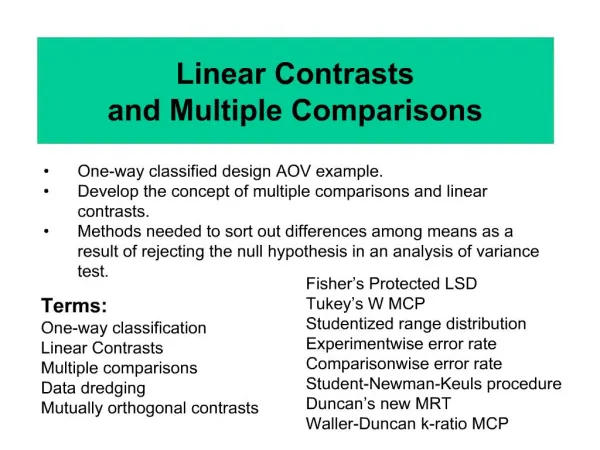
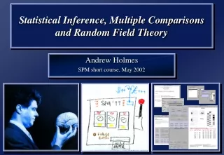
Multiple comparisons problem and solutions. James M. Kilner http://sites.google.com/site/kilnerlab/home. What is the multiple comparisons problem How can it be avoided Ways to correct for the multiple comparisons problem. a. b. Diff ?. a - b > 0. Problems.

E N D
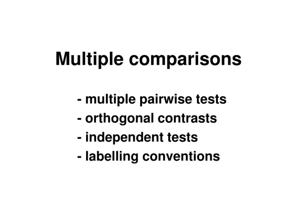
Multiple comparisons problem and solutions James M. Kilner http://sites.google.com/site/kilnerlab/home
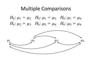
What is the multiple comparisons problem How can it be avoided Ways to correct for the multiple comparisons problem
a b
Diff ? a -b> 0
Problems MEG and EEG does not have zero dimensionality If one electrode data is at least one-dimensional If multiple electrodes data is at least three dimensions If time-frequency analysis then data can be four dimensional Massive multiple comparison problem
50 40 30 Frequency (Hz) 20 10 0 -1 0 1 2 Time (s) 1-D 2-D 3-D 2-D 2-D
Random Field Theory Contrast c
MCP example 2-D
Common Solutions One solution is to reduce the multi-dimensional data to zero-dimensional data by averaging over a window of interest This must be specified a priori or derived from an independent contrast. One can not base this window on where the effect is largest! ‘BUT the basic question remains - why would one do all this, and search for some odd effects this way, when it is all visible in the sensor level’
Bonferroni correction However, the data points in M/EEG data are not independent They are correlated either temporally, spatially or in frequency space
Random Field Theory Statistical parametric maps (e.g., t-maps) are fields with values that are, under the null hypothesis, distributed according to a known probability distribution. RFT is used to resolve the multiple comparisons problem that occurs when making inferences over the search-space: Adjusted p-values are obtained by using results for the expected Euler characteristic. At very high thresholds the Euler characteristic reduces to the number of suprathreshold peaks and the expected EC becomes the probability of getting a peak above threshold by chance. The expected EC therefore approximates the probability that the SPM exceeds some height by chance. The ensuing p-values can be used to find a corrected height threshold or assign a corrected p-value to any observed peak in the SPM.
Good lattice approximation? Will be true for high density recordings
No holes Zero or one blob
Expected Euler Characteristic 2D Gaussian Random Field • Ω: search region • λ(Ω) : volume • |Λ|1/2:roughness (1 / smoothness)
1 2 3 4 5 6 7 8 9 10 1 2 3 4 Smoothness Smoothness parameterised in terms of FWHM: Size of Gaussian kernel required to smooth i.i.d. noise to have same smoothness as observed null (standardized) data. FWHM Eg: 10 voxels, 2.5 FWHM, 4 RESELS The number of resels is similar, but not identical to the number independent observations. Smoothness estimated from spatial derivatives of standardised residuals: Yields an RPV image containing local roughness estimation.
Topological inference Topological feature: Peak height space uα non significant local maxima significant local maxima
Topological inference Topological feature: Cluster extent space uclus significant cluster non significant clusters
Topological inference Topological feature: Number of clusters space uclus Here, c=1, only one cluster larger than k.
Peak, cluster and set level inference Regional specificity Sensitivity Peak level test: height of local maxima Cluster level test: spatial extent above u Set level test: number of clusters above u
Random Field Theory • The statistic image is assumed to be a good lattice representation of an underlying continuous stationary random field. Typically, FWHM > 3 voxels (combination of intrinsic and extrinsic smoothing) • Smoothness of the data is unknown and estimated: very precise estimate by pooling over voxels ⇒ stationarity assumptions (esp. relevant for cluster size results). • RFT conservative for low degrees of freedom (always compare with Bonferroni correction). Afford littles power for group studies with small sample size.
Random Field Theory • A priori hypothesis about where an activation should be, reduce search volume ⇒ h • Volume Correction: • mask defined by (probabilistic) anatomical atlases • mask defined by separate "functional localisers" • mask defined by orthogonal contrasts • (spherical) search volume around previously reported coordinates
MCP example 2-D
Conclusion • There is a multiple testing problem and corrections have to be applied on p-values (for the volume of interest only (see SVC)). • Inference is made about topological features (peak height, spatial extent, number of clusters).Use results from the Random Field Theory. • Control of FWER(probability of a false positive anywhere in the image): very specific, not so sensitive. • Control of FDR (expected proportion of false positives amongst those features declared positive (the discoveries)): less specific, more sensitive.