Download
1 / 59
590 likes | 784 Views
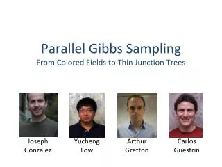
Parallel Gibbs Sampling From Colored Fields to Thin Junction Trees. Joseph Gonzalez. Yucheng Low. Arthur Gretton. Carlos Guestrin. Sampling as an Inference Procedure. Suppose we wanted to know the probability that coin lands “heads” We use the same idea for graphical model inference.

E N D
Parallel Gibbs SamplingFrom Colored Fields to Thin Junction Trees Joseph Gonzalez Yucheng Low Arthur Gretton Carlos Guestrin
Sampling as an Inference Procedure • Suppose we wanted to know the probability that coin lands “heads” • We use the same idea for graphical model inference “Draw Samples” Counts 4x Heads 6x Tails X1 Inference: X2 Inference: X3 X4 Graphical Model X5 X6
Terminology: Graphical Models • Focus on discrete factorized models with sparse structure: X1 f1,2 X2 Factor Graph f1,3 f2,4 X5 f2,4,5 X3 X4 f3,4 X1 X2 Markov Random Field X5 X3 X4
Terminology: Ergodicity • The goal is to estimate: • Example: marginal estimation • If the sampler is ergodic the following is true*: *Consult your statistician about potential risks before using.
Gibbs Sampling [Geman & Geman, 1984] • Sequentially for each variable in the model • Select variable • Construct conditional given adjacent assignments • Flip coin and updateassignment to variable Initial Assignment
Why Study Parallel Gibbs Sampling? “The Gibbs sampler ... might be considered the workhorse of the MCMC world.” –Robert and Casella • Ergodic with geometric convergence • Great for high-dimensional models • No need to tune a joint proposal • Easy to construct algorithmically • WinBUGS • Important Properties that help Parallelization: • Sparse structure factorized computation
From the original paper on Gibbs Sampling: “…the MRF can be divided into collections of [variables] with each collection assigned to an independently running asynchronousprocessor.” -- Stuart and Donald Geman, 1984. Converges to the wrong distribution!
The problem with Synchronous Gibbs • Adjacent variables cannot be sampled simultaneously. Strong Positive Correlation t=1 t=2 t=3 Heads: Tails: Strong Negative Correlation Sequential Execution t=0 Strong Positive Correlation Parallel Execution
Two Decades later • Same problem as the original Geman paper • Parallel version of the sampler is not ergodic. • Unlike Geman, the recent work: • Recognizes the issue • Ignores the issue • Propose an “approximate” solution • Newman et al., Scalable Parallel Topic Models.Jnl. Intelligen. Comm. R&D, 2006. • Newman et al., Distributed Inference for Latent Dirichlet Allocation. NIPS, 2007. • Asuncion et al., Asynchronous Distributed Learning of Topic Models. NIPS, 2008. • Doshi-Velez et al., Large Scale Nonparametric Bayesian Inference: Data Parallelization in the Indian Buffet Process. NIPS 2009 • Yan et al., Parallel Inference for Latent Dirichlet Allocation on GPUs. NIPS, 2009.
Two Decades Ago • Parallel computing community studied: Directed Acyclic Dependency Graph Sequential Algorithm Time Construct an Equivalent Parallel Algorithm Using Graph Coloring
Chromatic Sampler • Compute a k-coloring of the graphical model • Sample all variables with same color in parallel • Sequential Consistency: Time
Chromatic Sampler Algorithm For t from 1 to T do For k from 1 to K do Parfori in color k:
Asymptotic Properties • Quantifiable acceleration in mixing • Speedup: # Variables Time to updateall variables once # Colors # Processors Penalty Term
Proof of Ergodicity • Version 1 (Sequential Consistency): • Chromatic Gibbs Sampler is equivalent to aSequential ScanGibbs Sampler • Version 2 (Probabilistic Interpretation): • Variables in same color are Conditionally Independent Joint Sample is equivalent to Parallel Independent Samples Time
Special Properties of 2-Colorable Models • Many common models have two colorings • For the [Incorrect] Synchronous Gibbs Samplers • Provide a method to correct the chains • Derive the stationary distribution
Correcting the Synchronous Gibbs Sampler • We can derive two valid chains: t=1 t=2 t=3 t=4 Invalid Sequence t=0 t=0 t=1 t=2 t=3 t=4 t=5 Strong Positive Correlation
Correcting the Synchronous Gibbs Sampler • We can derive two valid chains: t=1 t=2 t=3 t=4 Invalid Sequence t=0 Chain 1 Strong Positive Correlation Converges to the Correct Distribution Chain 2
Theoretical Contributions on 2-colorable models • Stationary distribution of Synchronous Gibbs: Variables in Color 1 Variables in Color 2
Theoretical Contributions on 2-colorable models • Stationary distribution of Synchronous Gibbs • Corollary: Synchronous Gibbs sampler is correct for single variable marginals. Variables in Color 1 Variables in Color 2
From Colored Fields to Thin Junction Trees Chromatic Gibbs Sampler • Ideal for: • Rapid mixing models • Conditional structure does not admit Splash Splash Gibbs Sampler • Ideal for: • Slowly mixing models • Conditional structure admits Splash • Discrete models Slowly Mixing Models ?
Models With Strong Dependencies • Single variable Gibbs updates tend to mix slowly: • Ideally we would like to draw joint samples. • Blocking X2 Single site changes move slowly with strong correlation. X1
Blocking Gibbs Sampler • Based on the papers: • Jensen et al., Blocking Gibbs Sampling for Linkage Analysis in Large Pedigrees with Many Loops. TR1996 • Hamze et al., From Fields to Trees. UAI 2004.
An asynchronous Gibbs Sampler that adaptively addresses strong dependencies. Splash Gibbs Sampler
Splash Gibbs Sampler • Step 1: Grow multiple Splashes in parallel: ConditionallyIndependent
Splash Gibbs Sampler • Step 1: Grow multiple Splashes in parallel: Tree-width = 1 ConditionallyIndependent
Splash Gibbs Sampler • Step 1: Grow multiple Splashes in parallel: Tree-width = 2 ConditionallyIndependent
Splash Gibbs Sampler • Step 2: Calibrate the trees in parallel
Splash Gibbs Sampler • Step 3: Sample trees in parallel
Higher Treewidth Splashes • Recall: Tree-width = 2 Junction Trees
Junction Trees • Data structure used for exact inference in loopy graphical models fAB A fAB B A B D fAD fAD fBC fBC B C D D fCD C fCD fDE fCE fDE C D E E fCE Tree-width = 2
Splash Thin Junction Tree • Parallel Splash Junction Tree Algorithm • Construct multiple conditionally independent thin (bounded treewidth) junction trees Splashes • Sequential junction tree extension • Calibrate the each thin junction tree in parallel • Parallel belief propagation • Exact backward sampling • Parallel exact sampling
Splash generation • Frontier extension algorithm: Markov Random Field Corresponding Junction tree A A
Splash generation • Frontier extension algorithm: Markov Random Field Corresponding Junction tree A B B A
Splash generation • Frontier extension algorithm: Markov Random Field Corresponding Junction tree A B B C C B A
Splash generation • Frontier extension algorithm: Markov Random Field Corresponding Junction tree A B D B C D C B A D
Splash generation • Frontier extension algorithm: Markov Random Field Corresponding Junction tree A B D B C D C B A D E A D E
Splash generation • Frontier extension algorithm: Markov Random Field Corresponding Junction tree A B D B C D C B A D E A E F A D F E
Splash generation • Frontier extension algorithm: Markov Random Field Corresponding Junction tree A B D B C D C B A D E A E F D A G F A G E
Splash generation • Frontier extension algorithm: Markov Random Field Corresponding Junction tree A B D B C D C B H A D E A E F D A G F A G E B G H
Splash generation • Frontier extension algorithm: Markov Random Field Corresponding Junction tree A B D B C D C B H A B D E A BE F D A G F A B G E B G H
Splash generation • Frontier extension algorithm: Markov Random Field Corresponding Junction tree A B D B C D C B H A D E A E F D A G F A G E
Splash generation • Frontier extension algorithm: Markov Random Field Corresponding Junction tree A B D B C D C B H A D E A E F I D A G F D I A G E
Splash generation • Challenge: • Efficiently reject vertices that violate treewidth constraint • Efficiently extend the junction tree • Choosing the next vertex • Solution Splash Junction Trees: • Variable elimination with reverse visit ordering • I,G,F,E,D,C,B,A • Add new clique and update RIP • If a clique is created which exceeds treewidth terminate extension • Adaptive prioritize boundary C B H I D A G F E
Incremental Junction Trees 1 2 3 1 2 3 • First 3 Rounds: 4 5 6 4 5 6 4 4,5 2,5 {2,5,4} {5,4} 4 4,5 1 2 3 4 5 6 4 Junction Tree: {4} Elim. Order:
Incremental Junction Trees 1 2 3 • Result of third round: • Fourth round: 1 2 3 4 5 6 {2,5,4} {1,2,5,4} 4 5 6 4 4,5 2,5 Fix RIP 4 4 4,5 4,5 1,2,4 1,2,4 2,5 2,4,5
Incremental Junction Trees • Results from 4th round: • 5th Round: 1 2 3 {1,2,5,4} 4 5 6 1 2 3 {6,1,2,5,4} 4 5 6 4 4,5 2,4,5 1,2,4 4 4,5 5,6 2,4,5 1,2,4
Incremental Junction Trees • Results from 5th round: • 6th Round: {6,1,2,5,4} 1 2 3 1 2 3 {3,6,1,2,5,4} 4 5 6 4 5 6 1,2,3, 6 4 4,5 5,6 2,4,5 1,2,4 4 4,5 5,6 2,4,5 1,2,4
Incremental Junction Trees • Finishing 6th round: {3,6,1,2,5,4} 4 1,2,3,6 4 1,2,3,6 1 2 3 4,5 4,5 1,2,5,6 4 5 6 2,4,5 1,2,4 2,4,5 1,2,4 1,2,3, 6 1,2,5,6 1,2,5,6 4 1,2,3,6 4,5 2,4,5 1,2,4,5 4 4,5 5,6 2,4,5 1,2,4