Read : Ch. 17 in Electric Circuits, 9 th Edition by Nilsson Ch. 7 in Linear Systems and Signals, 2 nd

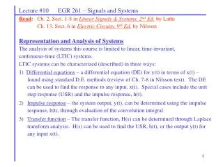
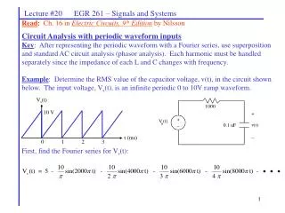
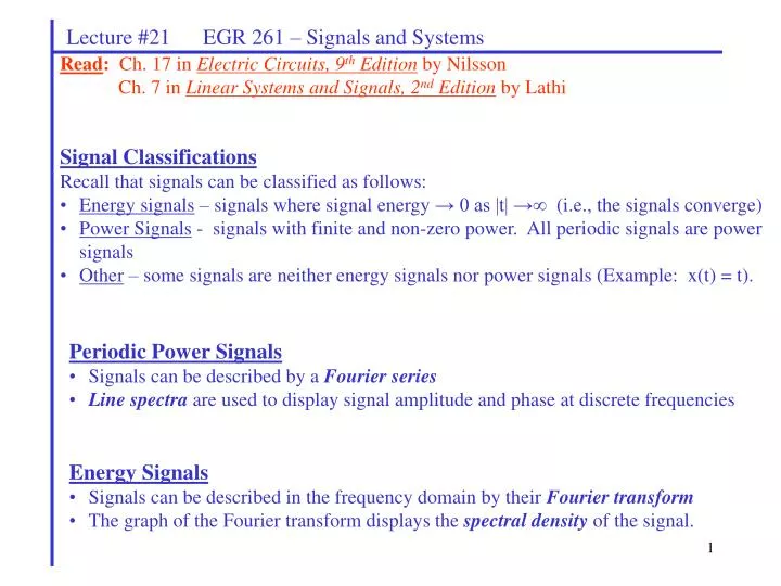
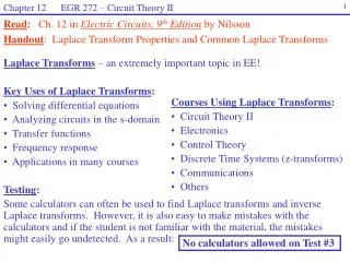
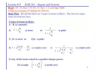
1. Lecture #21 EGR 261 – Signals and Systems Read: Ch. 17 in Electric Circuits, 9th Edition by Nilsson Ch. 7 in Linear Systems and Signals, 2nd Edition by Lathi • Signal Classifications • Recall that signals can be classified as follows: • Energy signals – signals where signal energy → 0 as |t| → (i.e., the signals converge) • Power Signals - signals with finite and non-zero power. All periodic signals are power signals • Other – some signals are neither energy signals nor power signals (Example: x(t) = t). • Periodic Power Signals • Signals can be described by a Fourier series • Line spectra are used to display signal amplitude and phase at discrete frequencies • Energy Signals • Signals can be described in the frequency domain by their Fourier transform • The graph of the Fourier transform displays the spectral density of the signal.

2. Lecture #21 EGR 261 – Signals and Systems Fourier Transforms The Fourier seriesrepresentation of a signal allowed us to describe a periodic signal in terms of its frequency domain properties of amplitude and phase (i.e., it line spectra). The Fourier transformallows us to describe the frequency domain properties of signals that are not periodic. The Fourier transform can be viewed as a special case of the bilateral (2-sided) Laplace transform where s = jw (i.e., σ = 0); however, the Fourier transform is more useful in certain communications and signal processing areas as it can be used to determine the spectral density of a signal. In the area of digital signal processing, continuous signals are sampled and represented by perhaps huge arrays of numbers. The frequency spectrum of such signals can be determined using Discrete Fourier Transforms (DFT’s). A shortcut method for determining the DFT is the Fast Fourier Transform (FFT). DFT’s and FFT’s are not covered in this course.

3. f(t) f(t) t t -/2 /2 0 -/2 /2 T 0 2T T→ --T Periodic Signal Period = T Aperiodic Signal T→ Lecture #21 EGR 261 – Signals and Systems Derivation of the Fourier Transform In addition to being related to the Laplace transform, the Fourier transform can be thought of as the limiting case of a Fourier series. Recall that the exponential Fourier series is written as: Allowing the fundamental period T to approach  changes a periodic function into an aperiodic function. Vm Vm As T →  then nwo → w and This integral is defined as the Fourier transform of f(t) and is denoted: Fourier transform

4. Lecture #21 EGR 261 – Signals and Systems Whereas the Fourier series of the pulse shown on the previous page yields a line spectrum showing signal amplitude (Cn) at discrete frequencies, the Fourier transform shows a continuous spectral density (CnT). Recall from last class that the Fourier series coefficients followed a sinc(x) function as shown below: Similarly, taking the Fourier transform of the aperiodic signal on the previous also yields a continuous spectrum following a sinc(x) function as shown to the right.

5. Lecture #21 EGR 261 – Signals and Systems Fourier Transform – the Limiting Case of the Fourier Series As another illustration that the Fourier transform is the limiting case of the Fourier series, consider how the line spectra becomes more dense as the period increases for the periodic waveforms shown in (a) – (c). As the period T → ∞, the spectrum becomes continuous as shown in (d). Reference: Figure 9-15, Transform Circuit Analysis for Engineering and Technology, 3rd Edition, by Stanley

6. Lecture #21 EGR 261 – Signals and Systems Inverse Fourier Transform Substituting the expression for CnT into the exponential Fourier series yields: As T→, CnT →F(w) and since T = 2π/w, 1/T →dw/2π, so Inverse Fourier transform

7. F f(t) F(w) time domain frequency domain) F-1 Lecture #21 EGR 261 – Signals and Systems Notation: F(w) = F {f(t)} = the Fourier transform of f(t). f(t) = F -1{F(w)} = the inverse Fourier transform of F(w). Uniqueness: Every f(t) has a unique F(w) and every F(w) has a unique f(t). Fourier transform Inverse Fourier transform

8. Lecture #21 EGR 261 – Signals and Systems Example: Find the Fourier transform of f(t) = e-atu(t) for a > 0. Also sketch |F(w)| versus w and (w) vs. w. Discuss using Excel or other programs to form these graphs.

9. Lecture #21 EGR 261 – Signals and Systems The Convergence of the Fourier Integral: A function f(t) has a Fourier transform if the integral definition of the Fourier transform below converges. The Dirichlet (pronounced “deer – clay”) conditions presented earlier regarding the existence of the Fourier series are sufficient, although not necessary, conditions to guarantee that the Fourier transform exists. The Dirichlet conditions are: 1) f(t) is single-valued 2) f(t) has a finite number of discontinuities 3) f(t) has a finite number of maxima and minima 4)

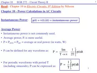
10. Lecture #21 EGR 261 – Signals and Systems Relationship between the Fourier transform and the Laplace transform: Earlier in the course we used the 1-sided or unilateral Laplace transform, defined as: 1-sided or unilateral Laplace transform (s =  + jw ) The 2-sided or bilateral Laplace transform is defined as: 2-sided or bilateral Laplace transform (s =  + jw ) The Fourier transform is essentially a special case of the Laplace transform where complex frequency is restricted to s = jw. Fourier transforms can be formed from a table of 1-sided Laplace transforms if all the poles of F(s) lie in the left half plane (LHP) of the s-plane. If F(s) has poles in the right half-plane or along the imaginary axis, the f(t) does not satisfy the constraint that Fourier transform (s = jw )

11. Lecture #21 EGR 261 – Signals and Systems Finding Fourier transforms from Laplace transforms: So the Fourier transform can be found from the Laplace transform if all poles of F(s) are in the left half plane (LHP). • Example: Consider the function f(t) = e-atu(t). • Find F(s), the Laplace transform of f(t). • Sketch the s-plane for F(s). • Find F(w) from F(s). Does it agree with the last example?

12. Lecture #21 EGR 261 – Signals and Systems Table of Laplace Transforms and Fourier Transforms This is not intended to be an extensive table of transforms, but serves to illustrate that the Fourier transform F(w) can sometimes be found from F(s) by replacing s with jw, but in other cases cannot.

13. Lecture #21 EGR 261 Table 7.1 - Fourier Transforms (from page 702 in Linear Signals & Systems, 2nd Edition, by Lathi) Discuss the difference between functions such as cos(wot) and cos(wot)u(t). The functions sgn(t) and rect(t/) will be defined shortly.

14. Lecture #21 EGR 261 – Signals and Systems Example: Find the Fourier transform of the function f(t) = u(t). u(t) 1 e-atu(t) (Example continued on next page) 0 t

15. Lecture #21 EGR 261 – Signals and Systems

16. Lecture #21 EGR 261 – Signals and Systems • Example: Find the Fourier transform of a constant, A. • Hint: Begin by finding the inverse Fourier transform of 2(w) using the integral definition. • Sketch the result (both f(t) and F(w)). • Does the result make sense? (Think of the constant as a DC value.)

17. Lecture #21 EGR 261 – Signals and Systems Example: Find the Fourier transform of cos(wot). Hint: Begin by finding the inverse transform of 2π(w-wo).

18. rect(t) 1 t 0 -1/2 1/2 rect(t/) 1 t -/2 0 /2 Lecture #21 EGR 261 – Signals and Systems Fourier Transforms of two important functions 1) rect(t) Earlier we saw that the Fourier transform of a pulse of width  and amplitude Vm was Vmsinc(w/2). This type of pulse is important and is sometimes referred to as a unit gate function or a gated pulse and is defined as follows:

19. Lecture #21 EGR 261 – Signals and Systems • Example: • If f(t) = 10rect(t/8), sketch f(t), find F(w), and sketch F(w). • If F(w) = 4sinc(w/16), sketch F(w), find f(t), and sketch f(t)

20. sgn(t) 1 t 0 -1 Lecture #21 EGR 261 – Signals and Systems Fourier Transforms of two important functions 2) sgn(t) The signum function (or sign function), sgn(t), is defined as follows: sgn(t) = u(t) – u(-t) To find the Fourier transform observe that sgn(t) + 1 = 2u(t) as shown to the right, so sgn(t) = 2u(t) - 1 sgn(t) + 1 = 2u(t) 2 0 t