Download
1 / 59
590 likes | 800 Views
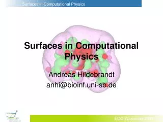
Surfaces in Computational Physics. Andreas Hildebrandt anhi@bioinf.uni-sb.de. What is computational physics?. Devoted to the numerical solution of „scientific problems“ Conceptually in between theoretical and mathematical physics Extremely broad range of topics and applications.

E N D
Surfaces in Computational Physics Andreas Hildebrandt anhi@bioinf.uni-sb.de
What is computational physics? • Devoted to the numerical solution of „scientific problems“ • Conceptually in between theoretical and mathematical physics • Extremely broad range of topics and applications All pictures from www.opendx.org
www.opendx.org www.scicomp.ucsd.edu/~mholst/ www.scicomp.ucsd.edu/~mholst/ www.vibroacoustics.co.uk/ Reasons for using (hyper-)surfaces in physics • Visualization, Graphical Analysis • Geometrization of Physics (c.f. General Relativity electrodynamics etc) • Speeding up expensive calculations • Specifying boundary conditions
(a) an electrostatic potential (b) a pressure field www.opendx.org www.scs.gmu.edu/~rlohner/ Visualization Visualizing scalar 3D fields has many important applications in computational physics like: 1. Coloring a surface with a scalar quantity like
quantum mechanical electron densities www.opendx.org Visualization Visualizing scalar 3D fields has many important applications in computational physics like: 2. Plotting the contour surface of a scalar quantity, e.g.
www.opendx.org Visualization Visualizing scalar 3D fields has many important applications in computational physics like: 3. Comparing different numerical methods graphical analysis of quantum mechanical basis sets
Geometrization of Physics Many modern concepts in physics are based on geometrical theories like e.g.: • General relativity: spacetime as a 4 dimensional Riemannian manifold, matter and energy yield the metric • Electrodynamics: electric and magnetic fields and fluxes as forms on a 3d manifold
Boundary Conditions • Theoretical physics describes the various phenomena encountered in nature quantitatively in the form of “theories” • These consist of one or more operator equations, connecting observable quantities of the system • Observables can be predicted from the knowledge of the others (e.g. electrostatic potential from charge density)
Boundary Conditions • Most „physical“ operators are differential or integro-differential operators, e.g. • LLaplace= D= r¢ r • LSchrödinger = H – i~¶t = –~2 (2m)(-1)D – i ~¶t • Solving a differential equation introduces integration constants ) to find a unique solution, their values have to be fixed by demanding that they fullfil „boundary conditions“
Boundary Conditions 3d–Problems ) specification of boundary conditions on a 2d–surface ) need a parameterization of boundary surfaces or as perturbation expansion about simple geometries ) analytical solutions only for simple geometries www.csd.abdn.ac.uk/~dritchie/ graphics/
Boundary Element Method (BEM) • Powerful tool for solving differential equations • Reduces the dimensionality of the problem • Applicable to arbitrary closed surfaces
Heat conduction Sound propagation urbana.mie.uc.edu/yliu/ Computational Fluid Dynamics wings.avkids.com Molecular Modeling www.opendx.org Medical imaging and modeling www.ccrl-nece.de/simbio Some applications for the boundary element method
Hot conducting side flux = ? Insulated side temperature = ? Insulated side temperature = ? temperature=? Cold conducting side flux=? Example: 2D steady state heat conduction Given a system with certain boundary temperatures and fluxes, compute the value of the temperature everywhere!
G3, u=100 W G2, q=0 G4, q=0 u = 0 G1, u=0 Example: 2D steady state heat conduction Given a system with certain boundary temperatures and fluxes, compute the value of the temperature everywhere! u = 0 )L = D u = temperature q = heat flux
E W Lu= 0 G The Boundary Element Method • Let L be a linear differential operator • We want to solve Lu = 0 in a domain W of a d-dimensional space E • Let G be the boundary of W in E
E Lū = R W Lu= 0 G • For the exactsolution u, we have Lu = 0 in W. • But numerically we can only expect to compute an approximation ū, so that Lū = R in W • R is called the residual of the equation • We can‘t hope for R=0, but we can try to find an particularly nice R!
E Lū = R W Lu= 0 G The residual R is a measure for the error of the numerical approximation. We can‘t make it disappear, but we can try to distribute the error over W so that it vanishes in a certain average sense:
The weighted residual • This integral is called a weighted residual • This is the starting point for many modern PDE solvers like the Finite Element Method (FEM) and the Boundary Element Method (BEM). These differ in their choice of w. • We have converted the differential equation Lū = 0 into an integro-differential equation with weaker continuity requirements and improved numerical stability
„Roadmap“ • For a given L, simplify the integro-differential equation and convert it into an integral equation • Choose a suitable w • Discretize W (FEM) or G (BEM) • Solve the simplified equation numerically on this discretization
Notational conventions • We’ll use the simplified Einstein convention: any repeated index denotes a summation over its whole range e.g.: • For the partial derivative with respect to xj, we use the comma convention: • Example:the Laplace equation:
Example: The Laplace Equation • The Laplace equation u,ii = 0 in W describes e.g. the electrostatic potential in the absence of charges, steady-state heat conduction, ... • It is a linear second order partial differential equation ) we need to specify two boundary conditions on G=¶W • We can e.g. specify the ‚temperature‘ u on GD (Dirichlet condition) and the ‚heat flux‘q = -ku,i on GN (Neumann condition), so that G = GD + GN
G3, u=100 W G2, q=0 G4, q=0 u,ii = 0 G1, u=0 A simple 2D example for steady state heat conduction: GN = G2 + G4 GD = G1 + G3 u,ii = 0 )L = D Weighted residual: In the following we will try to shift the derivatives from the unkown u to the known function w () integro-differential ! integral equation)
Integration by parts yields: And with the Gauß – divergence theorem (¶W =:G, n=surface normal) We arrive at Green‘s first identity:
Now we repeat the same steps for the domain integral on the rhs, which yields Green‘s second identity:
Note that the only differential of the unknown function u appearing here is the heat flux qi = u,i. qi only appears in the boundary integral over G. • In the Finite Element Method (FEM) we would now proceed by discretizing W (e.g. in a tetrahedron mesh), approximate u as a sum of piecewise polynomials on each element of the mesh and solve the above integral equation on the mesh using this approximation. • For many choices of L (including LLaplaceu = u,ii), there is a much more efficient technique available: if we know a fundamental solution or Green‘s function for L, we only have to compute integrals on the boundary G(Boundary Element Method, BEM)
The fundamental solution • For a given differential operator L, a fundamental solution or Green‘s function u* is given by the solution of the equation Lu* = -d(x, x) • d(x,x) is Dirac‘s delta distribution, defined by the property:
If we now choose w =u* – the fundamental solution of the Laplace operator – it follows: w ,ii = -d(x,x) • We define the scalar fluxes q = qi ni = u,i ni and q* = u*,i ni • Substituting this into the above equation, we obtain for all x2W / G: This representation formula yields the temperature inside , if the fundamental solution u* and the values of the heat flux and the temperature on the boundary are known. Only boundary integrals occur, and thus only the boundary needs discretization!
G3, u=100 W G2, q=0 G4, q=0 u,ii = 0 G1, u=0 This formula is only valid inside , i.e. in / . Unfortunately we only know the values of q(x) on N and the values of u(x) on D, so we have to find a way to compute the remaining unknown boundary values of u(x) (on N) and q(x) (on D).
The boundary integral equation • We need to find a way to compute u(x) and q(x) on the whole of consistent with the prescribed boundary conditions • The last derivation was only valid inside because the delta distribution (x,) is undefined if lies on the boundary of the integration domain • To avoid this problem, we extend the boundary around and let the size of this extension shrink to zero in a special limiting process
! 0 * ‘ ‘ = - * + Performing the limit!0, we can compute the integrals from the representation formula for the boundary terms. The integrals overare split according to = lim! 0 ‘= lim! 0{( - *) + }
Carrying out the integrals for the Laplace equation yields the boundary integral equation: Where is the Cauchy principle value of the integral. The computation of these integrals is cumbersome and highly dependent on the differential operator and the dimensionality of the system. Boundary Element Methods for Engineers and Scientists Gaul, Kögl, Wagner
For the Laplace equation in 2D we obtain with the fundamental solution the 2D Laplace boundary integral equation:
To solve this equation numerically, we discretize the boundary 1. We partition G into E boundary elements G(1),..., G(E), G = å G(i) 4 3 2 1
s 1 0 x y To solve this equation numerically, we discretize the boundary 2. Each Gi is mapped into a standard form. Instead of the coordinates {xI} of the reference frame, we use a simple parameterization {si} 4 3 2 1
To solve this equation numerically, we discretize the boundary 3. On each Gi, u(x) and q(x) are approximated polynomially The ûmi are the values of u at node m of element i. The polynomials Fm(s) are called shape function of node m of element i. Boundary Element Methods for Engineers and Scientists Gaul, Kögl, Wagner
q* u* • Discretization of : • !1+…+E Discretization of u and q: u(x), q(x) ! ui, qi
m m 1(s) 1 1 2(s) 1(s) s s 0 1 0 1 Node 1 Node 2 Boundary Elements in 2D In 2D, the boundary elements i are line elements. The degree of the interpolation (the degree of the polynomials m) is determined by the number of nodes per element (m)! Node 1 Constant elements (m=1) Linear elements (m=2)
G3, u=100 G3, û31=100 W 3 G2, q=0 G4, q=0 W u,ii = 0 Constant elements 4 2 G2, q21=0 G4, q41=0 u,ii = 0 G1, u=0 1 x G1, û11=0 Example y
Hli Gli • With this equation we can compute the unknown boundary values from the known boundary conditions • Then we can use the representation formula to compute u and q everywhere in • Several strategies exist for choosing the points that should be evaluated. We choose the collocation method: The equation above is evaluated only on the nodes of the discretization l (u(l)=:u(l)1)
Gli Hli Collocation reduces the boundary integral equation to a matrix equation: Hij and Gij only depend on the geometry, not on the values of u and q!
The Matrix Coefficients • The computation of the non-diagonal entries Hij, Gij i j is straight-forward • The diagonal terms Hii, Gii are a bit more difficult, since in these cases the integrand has a singularity in the integration domain! • This poses special problems to any numerical integration procedure on the boundary elements
G3, û31=100 3 W 4 2 G2, q21=0 G4, q41=0 u,ii = 0 1 x G1, û11=0
This can be solved easily if we move all unknown variables to the lhs of the equation: This yields:
û31=100, q31 = -75.77 Due to the symmetry, there is no lateral temperature gradient 3 Heat flows from the high to the low temperature W 4 2 u41=50,q41=0 u21=50,q21=0 u,ii = 0 1 x û11=0.00, q11 = +75.77
Hli Gli Temperature and heat flux for all points l inside the domain can now be computed from the representation formula: Note that all coefficients on the rhs are known, i.e. we don’t have to solve any additional equations! Computing the boundary integrals Hli and Gli suffices!
û31=100, q31 = -75.77 3 W 4 2 u41=50,q41=0 u21=50,q21=0 u,ii = 0 1 x û11=0.00, q11 = +75.77
s1 s1 3 4 3 1 s2 1 2 s2 2 Generalization to the 3D case Many of these techniques carry over to the 3 dimensional case. The most important changes are: 1) 2D triangular or quadrilateral elements replace the 1D line elements
Generalization to the 3D case Many of these techniques carry over to the 3 dimensional case. The most important changes are: 2) For each node we need tangential and normal vectors Boundary Element Methods for Engineers and Scientists Gaul, Kögl, Wagner
Generalization to the 3D case Many of these techniques carry over to the 3 dimensional case. The most important changes are: 3) For the numerical integration we need a mapping for the boundary elements to a local (s1, s2)2[0,1]£[0,1] orthogonal reference frame Boundary Element Methods for Engineers and Scientists Gaul, Kögl, Wagner