Distribution-free testing

1. Distribution-free testing If the data are normally distributed, we may apply a z-test or t-test when the parameter of interest is . But what if this is the normal probability plot: Or this:

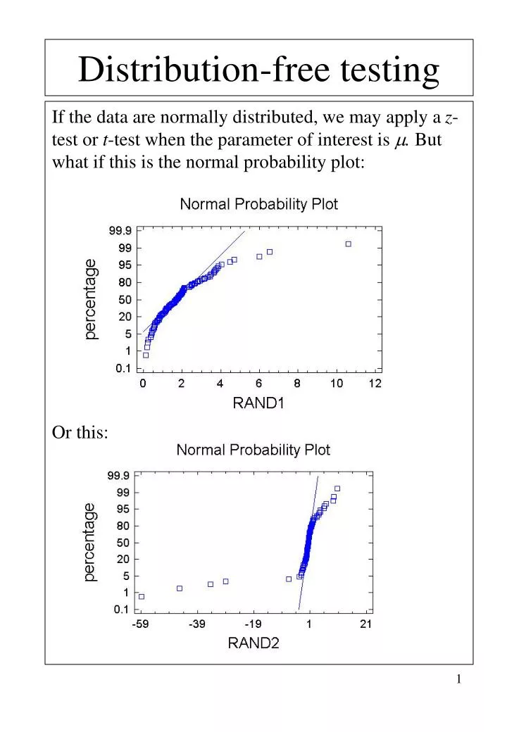
2. Distribution-free testing The Box-plots also indicate non-normality: skewness in the first case and more outliers than expected under normality in the second case:

3. Distribution-free testing When the data are clearly non-normal, we need an alternative: distribution-free testing. Also known under the terms: nonparametric testing or rank tests. Characteristic of such tests: they can be applied irrespective of what the true probability distribution of the data is (which we prove later). Disadvantage: the power of these tests is (slightly) smaller than those of normal-based tests if the data are normally distributed. Two of the most widely applied tests: Wilcoxon rank sum test: test H0 : 1 = 2 for two unpaired samples. Wilcoxon signed-rank test: Either one sample and test: H0 : = 0 or two samples, paired, test H0 : d= 0, with d= 1 -2.

4. Hypothesis testing, once again Steps of hypothesis testing 1. Parameter of interest (, 2, p)? Assumptions? Normal distribution, yes/no? 2. Hypotheses. One- or two-sided? 3. Testing with? a) Computer: p-values b) Table of critical values c) Asymptotic distribution of test statistic • Reject null hypothesis if a) p-value smaller or equal to  b) Value of test statistic lies in critical region. c) Asymptotic p-value is smaller or equal to 

5. Wilcoxon rank sum test • Parameter of interest:  = 1 -2 • H0 :  = 0 (or 1 =2). Alternative is either one- or two-sided • Computation of exact p- value with software (StatXact, Mathematica), tables of critical values are available in Statistisch Compendium (Dutch). Asymptotic normal distribution of the test statistic will be proven. 4. Reject null hypothesis if a) p-value smaller or equal to  b) Value of test statistic lies in critical region. c) Asymptotic p-value is smaller or equal to 

6. Wilcoxon rank sum test Test statistic 1: Rank the observations from small to large. Equal observations (ties) are assigned an average rank number (so, if the 4th, 5th and 6th observations are tied then they all correspond to rank (4+5+6) / 3 = 5. 2: Test statistic W: sum of ranks of the smallest sample, 34.5 in the example. 3: Find critical region for type I error . Note: for one-sided testing, first multiply  by 2 to obtain the critical value if the table is based on two-sided testing.

7. Wilcoxon rank sum test Smallest sample, sample ‘1’. The other is sample ‘2’. If • H1: 1 < 2 , use the left-critical value only b) H1: 1 > 2 , use right-crititical value only c) H1: 1  2 , use both. In the example (n = 5 and m = 6) for  = 0.05: a) look at  = 0.1: WL = 20, so reject H0 if W  20 b) WR = n(m + n + 1) –WL = 5*12 – 20 = 40. So, reject H0 if W  40 c) look at  = 0.05. WL = 18, WR = 42. Reject H0 if W  18 or W  42.

8. Wilcoxon rank sum test 4:Compare test statistic with critical region. One-sided testing (first protesis is a new design) : H1: 1 > 2 , because you want to show that the new protesis is better than the old one. W = 34.5 < 40 so do not reject H0: we cannot say that the new protesis is better than the old one. Later we show that for where c > 0, is standard normal distributed, so use this for values not in the Wilcoxon table.

9. Wilcoxon signed-rank test Situation: • One sample and test: H0 : = 0 • Two samples, paired, test H0 : d= 0, with d= 1 -2. In both cases we create one sample of which the mean should be approximately equal to ‘0’ if H0 holds. • Subtract specified 0 from each observation Data:3.9, 2.3, 4.0, 4.5, 1.5, 2.2, 1.7, 3.6, 6.1, 1.2, 5.3, 3.3, -0.6, 5.2, 0.2, 0.9, 2.6, 2.2, 3.4, 2.8 Hypothesis: H0:  = 2. Sample to which we will apply the test: Data:1.9, 0.3, 2.0, 2.5, -0.5, 0.2, -0.3, 1.6, 4.1, -0.8, 3.3, 1.3, -2.6, 3.2, -1.8, -1.1, 0.6, 0.2, 1.4, 0.8 b) Compute pairwise differences. These differences are the sample to which we will apply the test .

10. Wilcoxon signed-rank test Assumption: density f (x) of one-sample data is symmetric. Data: Before introducing a new beer on the market, the brewery wants to know whether people appreciate it more than an existing beer. Fifteen people give marks to both beers (blind test). The null hypothesis is H0 : d= 0, with d= nieuw – bestaand and the alternative hypothesis is H1 : d> 0.

11. Wilcoxon signed-rank test Data and ranks: Test statistic W+: sum of ranks corresponding to positive observations plus half of the sum of ranks corresponding to ‘0’. Ties: average the ranks. In the example: W+ = 99.

12. Wilcoxon signed-rank test Example Alternative hypothesis was H1 : d> 0, so one-sided test for  = 0.05. Right critical value WR = n(n+1) / 2 – WL = 120 – 30 = 90. W+ = 99 > WR = 90, so reject H0: d= 0: new beer is significantly nicer than the old beer. Normal approximation