Searching

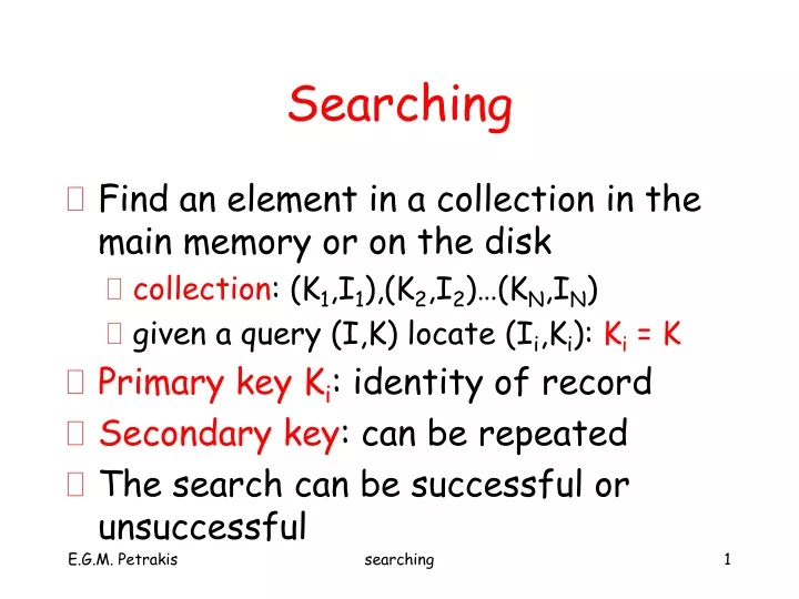
1. Searching • Find an element in a collection in the main memory or on the disk • collection: (K1,I1),(K2,I2)…(KN,IN) • given a query (I,K) locate (Ii,Ki): Ki = K • Primary key Ki: identity of record • Secondary key: can be repeated • The search can be successful or unsuccessful searching

2. Searching Methods • Sequential: data on lists or arrays • O(N) time, may be unacceptably slow • Indexed search: • tree indexing: data in trees • hashing or direct access : data on tables • Indexing requires preprocessing and extra space searching

3. Important Factors • Ordered or unordered data • Known or unknown data distribution • some elements are searched more frequently • Data in main memory or disk • time depends on algorithmic steps or disk accesses • Dynamic (or static) data collections • Insertions & deletions are allowed (or not allowed) • Types of search operations allowed • random queries: search for records with key = k • range queries: search for records keylow <= k <= keyhigh searching

4. Unordered Sequences • Lists or arrays of N elements • Number of comparisons: • pi: prob. to search for the i-th element • xi: number of comparisons when searching for the i-th element searching

5. Equally Probable Elements • Cost of successful search • Cost to search for an element which may or may not be in the array • if pe: probability to find it in the array searching

6. Other Cases • If p1 >= p2 >= … >= pN:move elements with higher probabilities to the front • Even if the probabilities are not known it is likely that some elements are searched more frequently than others searching

7. I. Move to Front • Move the element to the front • e.g., if the user searches for 10 • becomes: • Easy for lists, difficult for arrays: N-1 elements are moved 1 position to the left searching

8. II. Transpositions • The element is shifted one position to the right • e.g., search(10) • becomes • Easy for arrays and lists searching

9. Critique • Move to front adapts rapidly to the search conditions of the application • Transposition adapts slowly but is more intuitively correct • Combine the two techniques: • use initially move to front and • transposition later searching

10. Searching Ordered Sequences • Sort the elements once • complexity: O(logN) instead of O(N) • Search techniques: • binary search • interpolation search • indexed sequential search searching

11. I. Binary Search d=2 levels 2 3 4 5 8 9 10 d: max number of comparisons searching

12. Complexity • Maximum number or comparisons: a leaf is reached • Expected number of comparisons: tree searching stops before a leaf is reached: searching

13. II. Interpolation • Searching is guided by the values of the array • L: minimum value • U: maximum value • search position • Binary search always goes to the middle position searching

14. Example • if x[h] = key element found; else search array on the left or on the right of h • e.g. • search(80): focuses on the 20% rightmost part of the array searching

15. example pos=0 pos=9 Search for x=12: h=⎡(12-2+1)/(17-2)x10⎤=⎡110/15⎤=⎡7.3⎤8 A[8]=15 Search continues between A[0]=2 and A[7]=13 Search for x=12: h=⎡(12-2+1)/(170-2)x10⎤=⎡110/168⎤=⎡0.65⎤1 A[1]=3 Search continues between A[1]=3 and A[9]=170 Search for x=12: h=⎡(12-3+1)/(170-2)x9⎤=⎡110/168⎤=⎡0.65⎤1 A[2]=5 …. searching

16. Complexity • Average case: O(loglogN) uniform distribution of keys in the array • [3,5,8,10,13,15] • Worst case: O(N) on non uniform distribution • Searching for 9 in [1,2,3,4,5,6,7,8,9,100] will take 9 operations • Binary search is O(logN) always! searching

17. III. Indexed Sequential Search • A sorted index is set aside in addition to the array • Each element in the index points to a block of elements in the array • e.g., block of 10 or 20 elements • The index is searched before the array and guides the search in the array searching

18. array index searching

19. array index2 index1 searching

20. File Searching • Access a data page, load it in the main memory and search for the key • unordered files: O(#blocks) disk accesses • ordered files: O(log#blocks) disk accesses • disk head moves back and forth • difficult to control the disk head moves especially in multi-user environments • leave 20% extra space for insertions searching

21. file newfile transactions Ordered Files • Optimize the performance using an auxiliary batch file • batch operations in ascending key order • process the operations one after the other • batch a1 <= a2 <= … <=aN not searched searching

22. index (8, ) (16, ) (27, ) (38, ) (46, ) 5 8 10 1116 23 25 27 28 31 38 42 46 file Index Sequential Files (ISAM) • Random access based on primary key • Fast disk access through an index • Indices to data pages on the disk (block index) searching

23. overflow pages Overflows • No space left on track • Solutions • chaining: • distribution of overflow space between neighboring primary pages • file reorganization necessary soon or later!! • Dependence on hardware! • Pseudo dynamic behavior! searching

24. cylinder track or block surface ISAM Index • Cylinder index: one per disk unit • Master index: to disks - surfaces • Track index: one per cylinder searching

25. block search Key records cylinder index surface index Retrieval • Locate cylinder: 1st disk access • Locate surface: 2nd disk access • Locate track: 3rd disk access • Overflows will cause more disk accesses!! searching

26. ISAM • Data pages on the disk • Indices for faster retrievals • Static-Pseudo Dynamic Scheme • File re-organization will be needed soon in a dynamic environment • Dynamic Schemes • B-trees • B+-trees, … searching

27. Random Access Queries • Average and Worst Case Complexity: • Arrays, Lists: Sequential search O(N) • Shorted arrays: Binary search O(logN), static collection • Interpolation search: O(loglogN) but O(N) in the worst case, static collection only • Sorted lists: O(N) • Static Hashing: O(1) but O(N) in the worst case • Dynamic Hashing: O(1) • Binary Search Trees: O(logN), O(N) in the worst case • AVL trees: O(logN) searching

28. Range Queries • Basic idea: search for keylow, then search keys in order until keyhigh • Complexity depends on range: • If the range is not big (e.g. < 1%) compared to the range of keys in collection => complexity is that of a random query + complexity for the range • If the range is big => complexity is O(N) searching

29. Random Access Queries in Files • #blocks = N/sizeof(page) • Average and Worst Case Complexity: • Sequential files: O(#blocks) • Sorted search O(log#blocks) but O(#blocks) in the worst case (only static collection) • Static Hashing: O(1) but O(#blocks) in the worst case • Dynamic Hashing: O(1) always • B-trees, B+-tress: O(log#blocks) searching

30. Range Queries on Files • Basic idea: search for page with keylow, then search pages in order until the page with nd keyhigh is found • Complexity depends on range: • If the range is not big (e.g. < 1%) compared to the range of keys is collection => complexity is that of a random query + complexity for the range • If the range is big => complexity is O(#blocks) searching

31. searching

32. 10 15 25 5 2 18 20 Tree Search • The elements are stored in a Binary Search Tree searching

33. Complexity • Average number of key comparisons or length of path traversed • average case: O(logN) comparisons • worst case: BST is reduced to list and search is O(N) !! • The form of a BST depends on the insertion sequence • the keys are ordered: BST becomes list searching

34. α i N-i-1 < α >α Theorem • Testing for membership in a random BST takes O(logN) time (expected cost) • P(n): average number of nodes from root to a node • P(0)=0, P(1)=1 • P(i): average height of left sub-tree • P(n-i-1): average height of right sub-tree searching

35. Proof • Average number of comparisons • Average over all insertion sequences root left sub-tree right sub-tree searching

36. Proof (cont.) • … because a can be inserted first, second, n-th element => n cases • N – i - 1  i => • Prove by induction: P(N) <= 1 + 4logN • a more careful analysis shows that the constant is about 1.4 =>P(N) <= 1.4logN searching