Download
1 / 74
740 likes | 979 Views
Yarmouk University Faculty of Science . The Geometry of Generalized Hyperbolic Random Field. Hanadi M. Mansour. Supervisor: Dr. Mohammad AL-Odat. Abstract. Random Field Theory. The Generalized Hyperbolic Random Field. Simulation Study. Conclusions and Future Work. Abstract.

E N D
Yarmouk University Faculty of Science The Geometry of GeneralizedHyperbolic Random Field Hanadi M. Mansour Supervisor: Dr. Mohammad AL-Odat
Abstract Random Field Theory The Generalized Hyperbolic Random Field Simulation Study Conclusions and Future Work
Abstract • In this thesis, we introduce a new non-Gaussian random field called the generalized hyperbolic random field. • We show that the generalized hyperbolic random field generates a family of random fields. • We study the properties of this field as well as the geometry of its excursion set above high thresholds. • We derive the expected Euler characteristic of its excursion set in a close form.
Abstract –Cont. • Also we find an approximation to the expected number of its local maxima above high thresholds. • We derive an approximation to size of one connected component (cluster) of its excursion set above high threshold. • We use simulation to test the validity of this approximation. Finally we propose some future work. BACK
Chapter Two Random Field Theory
Random Field Theory • In this chapter, we introduce to the random field theory and give a brief review of literature. • Most of the material covered in this chapter is based on Adler (1981), Worsely (1994) and Alodat (2004).
Random fields • We may define the random field as a collection of random variables together with a collection of measures or distribution functions.
Random fields –Cont. • A Gaussian random field (GRF) with covariance function R( s, t ) is stationary or homogenous if its covariance function depends only on the difference between two points t, sas follows: R ( s , t ) = R ( s– t ) • And is isotropic if its covariance function depends only on distance between two points t, sas follows: R ( s , t ) = R ( ║t – s║)
Excursion set • Let be a random field. For any fixed real number u and any subset we may define the excursion set of the field X (t) above the level u to be the set of all points for t Є C which X (t) ≥ u • i.e.; the excursion set Au (X) = Au(X , C) = {t Є C : X (t) ≥ u}
Excursion set – Cont. • If X (t) is a homogeneous and smooth Gaussian random field, then with probability approaching one as , the excursion set is a union of disjoint connected components or clusters such that each cluster contains only one local maximum of X (t) at its center.
Expectation of Euler characteristic • The Euler characteristic simply counts ( the number of connected components) - (number of holes) in Au (Y) • As u gets large, these holes disappear, and as a result the Euler characteristic counts only the number of connected components. • According to Hasofer (1978), the following approximation is accurate.
Expectation of Euler characteristic – Cont. • Adler (1981) derived a close form of the Expectation of Euler characteristic when the random field is a Gaussian as the following: Where: .
Euler characteristic intensity • Let be an isotropic random field. Cao and Worsley (1999) define , the jth Euler characteristic intensity of the field by
Euler characteristic intensity –Cont. • Cao and Worsley (1999) are give the values of for j = 0, 1, 2, 3 when the random field is a Gaussian. • Also, they give the following approximation
Expectation of the number of local maxima • For a random field Y (t) above the level u. • Let denote the number of local maxima. • Adler (1981) gives the following formula if the random field is a Gaussian • As it follows that
Expected volume of one cluster using the PCH • Poisson clumping heuristic (PCH) technique can be employed to find an approximation to the mean value of the volume of one cluster to get the following approximation for
Distribution of the maximum cluster volume • In this section, we will describe how to approximate of the maximum volume of the clusters of the excursion set of a stationary random field Y (t) using the Poisson clumping heuristic approach given by Aldous(1989). • The same procedure was adopted by Friston et al. (1994) to find the distribution of the maximum volume of the excursion set of a single Gaussian random field.
Distribution of the maximum cluster volume –Cont. • Then we have the following formula for the distribution of the maximum cluster BACK
Chapter Three The Generalized Hyperbolic Random Field (GHRF)
The Generalized Hyperbolic Random Field (GHRF) • Let be a Gaussian random field with zero mean and variance equal to one, also let W be a generalized inverse Gaussian random variable independent of . • We define the Generalized Hyperbolic Random Field (GHRF) by: Where:
Generalized hyperbolic distribution (GHD) • A random vector Y is said to have a d- dimensional generalized hyperbolic distribution with parameters if and only if it has the joint density Where
Generalized hyperbolic distribution (GHD) – Cont. • We note that the generalized hyperbolic distribution is closed under marginal and conditioning distributions, also it is easy to see that it is closed under affine transformation.
Some special cases • We derive from the generalized hyperbolic distribution the following distributions: • The one dimensional normal inverse Gaussian (NIG) distribution. • The one - dimensional Cauchy distribution • The variance Gamma distribution. • The d-dimensional skewed t distribution. • The d-dimensional student t distribution.
Properties of GHRF • The isotropy of . • The is also continuous in mean square sense. • The is almost surely continuous at t*. • The GHRF has the mean square partial derivatives in the ith direction at t. • The GHRF is ergodic.
Properties of GHRF -Cont. • For every k and every set of points t1,…,tk C the vector has a multivariate generalized hyperbolic distribution. • Differentiability of implies the differentiability of • The mean and covariance functions of the GHRF are:
Expectation of Euler characteristicof (GHRF) • In this section we derive the Expectation of Euler characteristic when the random field generalized hyperbolic random field. • Theorem: • The Expected Euler characteristic of is given by:
Expectation of Euler characteristicof (GHRF) – Cont. • Then we obtain the following formula:
Expectation of Euler characteristicof (GHRF) – Cont. • Where
Euler characteristic intensity of Y(t) • Theorem • For the GHRF the jth Euler characteristic intensity of is given by: • Based on the previous theorem we have found the values of for j = 0, 1, 2 and 3 in our work.
Expected number of local maximaof Y(t) • Since W varies from 0to ∞ then we cannot obtain a close form for the expectation of the number of local maxima, but we will obtain the expected number of local maxima of by separating into two parts as follows:
Expected number of local maximaof Y (t) –Cont. • We ignore the second term from the above integral if a is large enough, then we approximate • And we get the following approximation
Size distribution of one component • In this section, we derive an approximation to the distribution of the size of one connected component of . • When To do this, we approximate the field near a local maximum at t = 0 by the quadratic form
Size distribution of one component -Cont. • The cluster size (the size of one connected component of ) is approximated by V the volume of the d-dimensional ellipsoid • Where:
Mean volume of one cluster using PCH • In this section ,we will derive approximation to the mean value of the volume of one cluster of the excursion set of using Poisson clumping heuristic.
Mean volume of one cluster using PCH -Cont • For d = 2 we get the approximation formula BACK
Chapter Four Simulation Study
Comparing the exact and the approximate distributions • The following figuresshow the simulation results for different values of , FWHM, grid, and λ.
Empirical distributions F and G of V at different thresholds for: Fig: 4.1
Empirical distributions F and G of V at different thresholds for: Table: 1
Empirical distributions F and G of V at different thresholds for: Fig: 4.3
Empirical distributions F and G of V at different thresholds for: Table: 3
Empirical distributions F and G of V at different thresholds for: Fig: 4.4
Empirical distributions F and G of V at different thresholds for: Table: 4
Empirical distributions F and G of V at different thresholds for: Fig: 4.7
Empirical distributions F and G of V at different thresholds for: Table: 7
Empirical distributions F and G of V at different thresholds for: Fig: 4.8
Empirical distributions F and G of V at different thresholds for: Table: 8
Empirical distributions F and G of V at different thresholds for: Fig: 4.10
Empirical distributions F and G of V at different thresholds for: Table: 10
Empirical distributions F and G of V at different thresholds for: Fig: 4.11