Download
1 / 48
520 likes | 695 Views
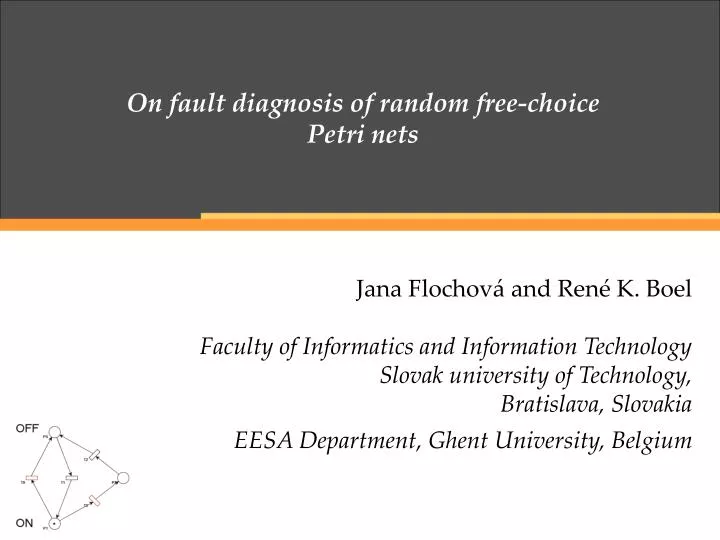
On fault diagnosis of random free-choice Petri nets. Jana Flochová and René K. Boel F aculty of Informatics and Information Technology Slovak university of Technology, Bratislava, Slovakia EESA Department, Ghent University, Belgium. Outline of the presentation.

E N D
On fault diagnosis of random free-choicePetri nets Jana Flochová and René K. Boel Faculty of Informatics and Information Technology Slovak university of Technology, Bratislava, Slovakia EESA Department,Ghent University, Belgium
Outline of thepresentation • Models, diagnosis of DES based on Petri net models • Minimal context and explanations – (Jiroveanu, Boel, Bordbar 2008) • Probabilistic (random) free choice Petri nets • Calculation of likelihood values for minimal explanations; probabilities of failures • Deterministic analysis of the past, probabilistic analysis of the future • Examples
Outline of thepresentation • Models, diagnosis of DES based on Petri net models • Minimal context and explanations – (Jiroveanu, Boel, Bordbar 2008) • Probabilistic (random) free choice Petri nets • Calculation of likelihood values for minimal explanations; probabilities of failures • Deterministic analysis of the past, probabilistic analysis of the future • Examples • Conclusions
Outline of thepresentation • Models, diagnosis of DES based on Petri net models • Minimal context and explanations – (Jiroveanu, Boel, Bordbar 2008) • Probabilistic (random) free choice Petri nets • Calculation of likelihood values for minimal explanations; probabilities of failures • Deterministic analysis of the past, probabilistic analysis of the future • Examples • Conclusions
Outline of thepresentation • Models, diagnosis of DES based on Petri net models • Minimal context and explanations – (Jiroveanu, Boel, Bordbar 2008) • Probabilistic (random) free choice Petri nets • Calculation of likelihood values for minimal explanations; probabilities of failures • Deterministic analysis of the past, probabilistic analysis of the future • Examples • Conclusions
Outline of thepresentation • Models, diagnosis of DES based on Petri net models • Minimal context and explanations – (Jiroveanu, Boel, Bordbar 2008) • Probabilistic (random) free choice Petri nets • Calculation of likelihood values for minimal explanations; probabilities of failures • Deterministic analysis of the past, probabilistic analysis of the future • Examples • Conclusions
Outline of thepresentation • Models, diagnosis of DES based on Petri net models • Minimal context and explanations – (Jiroveanu, Boel, Bordbar 2008) • Probabilistic (random) free choice Petri nets • Calculation of likelihood values for minimal explanations; probabilities of failures • Deterministic analysis of the past, probabilistic analysis of the future • Examples • Conclusions
Outline of thepresentation • Models, diagnosis of DES based on Petri net models • Minimal context and explanations – (Jiroveanu, Boel, Bordbar 2008) • Probabilistic (random) free choice Petri nets • Calculation of likelihood values for minimal explanations; probabilities of failures • Deterministic analysis of the past, probabilistic analysis of the future • Examples • Conclusions
Outline of thepresentation • Models, diagnosis of DES based on Petri net models • Minimal context and explanations – (Jiroveanu, Boel, Bordbar 2008) • Probabilistic (random) free choice Petri nets • Calculation of likelihood values for minimal explanations; probabilities of failures • Deterministic analysis of the past, probabilistic analysis of the future • Examples • Conclusions
Models – Petri Nets 4) M0 : P N is the initial marking <, #, denote precedence, conflict, concurrency relations of nodes A free-choice Petri netis a restricted class where every arc from a place to a transition is either the unique output arc from that place, or a unique input arc to the transition.
Models – Petri Nets An occurrence netOis a netO= (B, E,), with the elements of B called conditions, those of E called events, satisfying following properties xBE[x x] (no node is in self conflict) xBE[x < x] (is a partial order, acyclic) xBE{y: y < x}< (is well-formed) bB:b 1 (b denotes the set of input elements of b => each place has at most one input transition, no backward conflict). A configurationC=(Bc, Ec,) is a subset of O, which is: conflict free (no two nodes are in conflict), causally upward-closed (ifx´<1x,and xC, then x´C), and min(C) min (O).
Diagnosis based on PN – problem statement We consider the following structural and functional assumptions: • The overall plant model is bounded (possibly well formed free-choice) • The initial marking M0is precisely known, the set of transitions T = To Tuo • The plant observation is represented by a subset of observable transitions • The occurrence of an observable transition To is always reported correctly and without delays • No design-error assumptions
Diagnosis based on PN – problem statement We consider the following structural and functional assumptions: • The overall plant model is bounded (possibly well formed free-choice) • The initial marking M0is precisely known, the set of transitions T = To Tuo • The plant observation is represented by a subset of observable transitions • The occurrence of an observable transition To is always reported correctly and without delays • No design-error assumptions
Diagnosis based on PN – problem statement We consider the following structural and functional assumptions: • The overall plant model is bounded (possibly well formed free-choice) • The initial marking M0is precisely known, the set of transitions T = To Tuo • The plant observation is represented by a subset of observable transitions • The occurrence of an observable transition To is always reported correctly and without delays • No design-error assumptions
Diagnosis based on PN – problem statement We consider the following structural and functional assumptions: • The overall plant model is bounded (possibly well formed free-choice) • The initial marking M0is precisely known, the set of transitions T = To Tuo • The plant observation is represented by a subset of observable transitions • The occurrence of an observable transition To is always reported correctly and without delays • No design-error assumptions
Diagnosis based on PN – problem statement We consider the following structural and functional assumptions: • The overall plant model is bounded (possibly well formed free-choice) • The initial marking M0is precisely known, the set of transitions T = To Tuo • The plant observation is represented by a subset of observable transitions • The occurrence of an observable transition To is always reported correctly and without delays • No design-error assumptions
Diagnosis based on PN – problem statement We consider the following structural and functional assumptions: • The overall plant model is bounded (possibly well formed free-choice) • The initial marking M0is precisely known, the set of transitions T = To Tuo • The plant observation is represented by a subset of observable transitions • The occurrence of an observable transition To is always reported correctly and without delays • No design-error assumptions
Diagnosis based on PN – problem statement Faulty behaviour Normal behaviour Faults Tf are represented by a subset Tf Tuo of unobservable (silent transitions – ( due e.g. limited sensor information ) A fault or an unreliable sensor (when some messages may become lost) can be modelled provided that another unobservable transition is included in the model "in parallel" to the observable transition
Diagnosis based on PN – problem statement G. Jiroveanu, R.K. Boel, and B. Bordbar. On-Line Monitoring of Large Petri Net Models Under Partial Observation. Journal Discrete Event Dynamic Systems, 2008 Minimal context, minimal explanation, minimal marking.
Probabilistic settings • The probability of firing a transition should not depend on what concurrent transitions do, and the order on which concurrent transitions fire should not be randomized • Firing should not necessarily be reduced to one transition at a time. • The probability of firing a given transition dependsonly on its own recourses.
0,7 0,05 0,25 Probabilistic settings
Probabilistic settings The probability function on the set of configurations is defined as follows
Probabilistic settings • A stochastic analysis of faults that either occurred in the past or that may occur in the future prior to the next observed event occurrence (Flochová et al. 2007); so that the explanation only includes unobservable future events not belonging to the minimal explanations. • A deterministic analysis of faults that must have occurred in the past (Jiroveanu, Boel, Berdbar 2008) and a probabilistic analysis of faults that may occur in the future prior to the next observed event occurrence.
Probabilistic settings Having the set of minimal configurations C(On), respectivelythe set of minimal explanations of the received observationsLN(On) is defined
Probabilistic settings Having the set of minimal configurations C(On), respectivelythe set of minimal explanations of the received observationsLN(On) is defined The plant diagnosis after observing On based on the setof minimal explanations - obtained by projecting the set ofminimal explanations onto the set of fault events
Probabilistic settings Having the set of minimal configurations C(On), respectivelythe set of minimal explanations of the received observationsLN(On) is defined The plant diagnosis after observing On based on the setof minimal explanations - obtained by projecting the set ofminimal explanations onto the set of fault events
Probabilistic settings Having the set of minimal configurations C(On), respectivelythe set of minimal explanations of the received observationsLN(On) is defined The plant diagnosis after observing On based on the setof minimal explanations - obtained by projecting the set ofminimal explanations onto the set of fault events
Probabilistic settings All explanations - similar expressions after removing all underscores.
Probabilistic settings • Steps needed in order to derive fault probabilities: • Compute the set of minimal explanations of the most recent observed event. Derive minimal explanations of the last observed event t0 and minimal explanations of a sequence of observed events. • (2) Compute the unnormalized probability of all minimal explanations • (3) Sort explanations in descending order starting from the most probable ones. Shellsort can be used, branch and bound like improvements can be useful in order to avoid enumerating very unlikely explanations. • (4) Accept top x % (0-100 %) of explanations according to the input requirements. • (5) Compute the set of maximal explanations of the most recent observed event, if required.
Probabilistic settings (6) Compute the unobservable continuations, which follow after the next observable transitions and partition the continuations into the following sets: the set of configurations, which contain at least a faulty event; a set of configurations, which contain at least a faulty event of the fault of the type i; and the set of configurations, which don’t contain any faulty event. A modification of classical AI depth search, which evaluates at first the node that has the most nodes between itself and the last observed transition, can be used for computing the set of continuations equipped with probabilities.
Probabilistic settings (7) Compute the unnormalized probabilities of the faults (faults of the type i) of all continuations (of unobservable reaches after the last observation). (8) Compute the unnormalized probabilities of the faults (faults of the type i) based on the sets of all explanations. (9) Normalize the probabilities
Laboratory example- older Fischertechnik-modelold unreliable sensors and all parts, AB PLC control
!!!!Possibly a model, shortly Minimal explanations of the last event
Conclusions Two methods of probabilistic diagnosis were presented, both methods use minimal explanations and contexts concept, probabilities assigned to conflicting transitions and , reverse Petri nets. They both are based on [George and you] or better [George, you and Bordbar], and [Benveniste et al.] approaches. • 1. the method uses the probabilistic analysis of the plant evolution before the last observed event and the probabilistic estimation of the future evolution of the plant after the last observed event [NYC]. • 2. The second method (novel approach) is based on the deterministic analysis of the plant evolution before the last observed event and the probabilistic estimation of the possible future failure evolution of the plant.
Conclusions Two methods of probabilistic diagnosis were presented, both methods use minimal explanations and contexts concept, probabilities assigned to conflicting transitions and , reverse Petri nets. They both are based on [George and you] or better [George, you and Bordbar], and [Benveniste et al.] approaches. 1st method uses the probabilistic analysis of the plant evolution before the last observed event and the probabilistic estimation of the future evolution of the plant after the last observed event [NYC]. • 2. The second method (novel approach) is based on the deterministic analysis of the plant evolution before the last observed event and the probabilistic estimation of the possible future failure evolution of the plant.
Conclusions Two methods of probabilistic diagnosis were presented, both methods use minimal explanations and contexts concept, probabilities assigned to conflicting transitions and , reverse Petri nets. They both are based on [George and you] or better [George, you and Bordbar], and [Benveniste et al.] approaches. 1st method uses the probabilistic analysis of the plant evolution before the last observed event and the probabilistic estimation of the future evolution of the plant after the last observed event [NYC]. 2nd method (a novel approach) is based on the deterministic analysis of the plant evolution before the last observed event and the probabilistic estimation of the possible future failure evolution of the plant.
Advantages of the approach • The probabilistic setting allows us to incorporate statistical knowledge: on the production of faults: some event may be more likely than the others depending on reliability tests on devices, on the previous experience on monitoring the plant or the network (relative frequencies of spontaneous faults), on the loss of information on faults (e.g. masking of an alarm, temporally unavailable links, faults of protocols). • Methods allow some smoothness of observation, i.e. including of misleading observations and not observing of a normally observable events in the model. • Randomization of the model also provides a convenient way of introducing robustness of the model against modeling errors on faults propagation.
Problems and open questions • The process of randomization has to be done very carefully and one has to tackle several problems in assigning probabilities. • Decentralized diagnosis algorithms and distributing setting are needed to allow fault detection in large plants possible solution - several communicating probabilistic Petri nets components computing local probability assignment for all locally possible traces explaining observations. • components can interact by exchanging tokens via boundary places (or boundary synchronizing transitions), common normalization for both interacting component; • Relaxing the assumption of well formed free choice Petri nets following [Haar 2003]
Benveniste, A. et al.: “Fault detection and diagnosis in distributed systems: an approach bypartially stochastic Petri nets.” Discrete Event Dynamic Systems: Theory and Applications, vol. 8, pp. 203-231, June 1998. • A. Benvensite, E. Fabre, and S. Haar. Markov nets: Probabilistic models for distributed and concurrent systems. IEEE Transactions on Automatic Control, 48(11):1936–1950, 2003. • Benveniste, A. et al.: “Diagnosis of asynchronous discrete event systems, a net unfolding approach.” IEEE Transactions on Automatic Control, 48(5), pp. 714-727, May 2003. • S. Haar, ”Probabilistic cluster unfoldings for Petri nets”,Technical report 1517, IRISA, Rennes, France, 2003. • J. Esparza. S. Romer and W. Vogler. An improvement of McMillan’s unfolding algorithm. Lect. Notes in Computer Science 1055, 87–106, Springer-Verlag, 1996. • J. Flochova, R. K. Boel, and G. Jiroveanu. On Probabilistic Diagnosis for Free-Choice Petri Nets. Proceeding of ACC, NYC, US, 5655–5656, 2007. • G. Jiroveanu, R.K. Boel, and B. Bordbar. On-Line Monitoring of Large Petri Net Models Under Partial Observation. Journal Discrete Event Dynamic Systems, 18:323–354, 2008. • M. Nielsen, G. Plotkin, and G. Winskel. Petri nets, event structures and domains, part I. Theoret. Computer Science, 13:85–108, 1981.