Download
1 / 37
370 likes | 536 Views
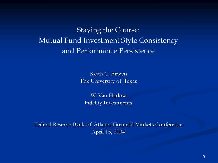
Staying the Course: Mutual Fund Investment Style Consistency and Performance Persistence. Keith C. Brown The University of Texas W. Van Harlow Fidelity Investments Federal Reserve Bank of Atlanta Financial Markets Conference April 15, 2004. Research Premise.

E N D
Staying the Course: Mutual Fund Investment Style Consistency and Performance Persistence Keith C. Brown The University of Texas W. Van Harlow Fidelity Investments Federal Reserve Bank of Atlanta Financial Markets Conference April 15, 2004
Research Premise Does Investment Style Consistency Impact Performance? Higher Style Consistency Lower Style Consistency Cap: Small to Large (%) Cap: Small to Large (%) Value to Growth (%) Value to Growth (%)
Why Style Consistency Might Matter • Fund Outflows Due to Style Drift • Inability of Plan Sponsors to Identify Manager’s Style • Higher Consistency = Lower Turnover? • Possibility of Lower Transaction Costs and Expense Ratios • Style Timing Might be a “Loser’s Game” • Analog to Difficulty of Successful Tactical Asset Allocation • Style Consistency as a Possible “Signal” of Superior Manager Performance
Higher Returns for More Style Consistent Funds Large Growth Mid Value Mid Blend Mid Growth Small Value Small Blend Small Growth Simple Evidence Average Annual Return (1991-2000) Peer Group Style Consistency Large Value Lower 11.10% Higher 13.05% Large Blend Lower 16.69% Higher 20.04% Lower 18.55% Higher 19.86% Lower 17.30% Higher 13.58% Lower 12.95% Higher 12.86% Lower 13.90% Higher 15.44% Lower 15.83% Higher 16.65% Lower 14.28% Higher 15.62% Lower 12.78% Higher 14.21%
Large Value 47.50% 45.50% 77.00% 38.00% Large Growth 68.00% 60.50% Mid Value 63.00% 60.00% Mid Blend 63.00% 39.59% Mid Growth 115.00% 76.00% Small Value 50.00% 44.82% 84.50% 47.00% Small Growth 89.00% 78.00% Complicating Factors Median Annual Fund Return (1991-2000) Higher Returns for More Style Consistent Funds Peer Group Style Consistency Median Turnover Median Expense Ratio Lower 11.10% 1.22% Higher 13.05% 1.02% Large Blend Lower 16.69% 1.25% Higher 20.04% 0.93% Lower 18.55% 1.36% Higher 19.86% 1.07% Lower 17.30% 1.40% Higher 13.58% 1.16% Lower 12.95% 1.41% Higher 12.86% 1.23% Lower 13.90% 1.40% Higher 15.44% 1.29% Lower 15.83% 1.39% Higher 16.65% 1.15% Small Blend Lower 14.28% 1.50% Higher 15.62% 1.12% Lower 12.78% 1.46% Higher 14.21% 1.33%
Large Value 47.50% 45.50% 77.00% 38.00% Large Growth 68.00% 60.50% Mid Value 63.00% 60.00% Mid Blend 63.00% 39.59% Mid Growth 115.00% 76.00% Small Value 50.00% 44.82% 84.50% 47.00% Small Growth 89.00% 78.00% Complicating Factors Median Annual Fund Return (1991-2000) Higher Returns for More Style Consistent Funds Peer Group Style Consistency Median Turnover Median Expense Ratio Lower 11.10% 1.22% Higher 13.05% 1.02% Large Blend Lower 16.69% 1.25% Higher 20.04% 0.93% Lower 18.55% 1.36% Higher 19.86% 1.07% Lower 17.30% 1.40% Higher 13.58% 1.16% Lower 12.95% 1.41% Higher 12.86% 1.23% Lower 13.90% 1.40% Higher 15.44% 1.29% Lower 15.83% 1.39% Higher 16.65% 1.15% Small Blend Lower 14.28% 1.50% Higher 15.62% 1.12% Lower 12.78% 1.46% Higher 14.21% 1.33%
Past Literature • Investment Style Appears to Matter • Fund Objectives: McDonald (JFQA, 1974); Malkiel (JF, 1995) • Security Characteristics: Basu (JF, 1977); Banz (JFE, 1981); Fama and French (JF, 1992; JFE, 1993) • Style Premiums: Capaul, Rawley, Sharpe (FAJ, 1993); Lakonishok, Shleifer, Vishny (JF, 1994); Fama and French (JF, 1998); Chan and Lakonishok (FAJ, 2004); Phalippou (Working Paper, 2004) • Style Definitions: Roll (HES, 1995); Brown and Goetzmann (JFE, 1997) • Style Rotation: Barberis and Shleifer (JFE, 2003) • Fund Performance Persistence • Classic Study: Jensen (JF, 1968) • Hot & Icy Hands: Grinblatt and Titman (JF, 1992); Hendricks, Patel, Zeckhauser (JF, 1993); Brown and Goetzmann (JF, 1995); Elton, Gruber, Blake (JB, 1996), Ibbotson and Patel (Working Paper, 2002) • Accounting for Momentum: Jegadeesh and Titman (JF, 1993); Carhart (JF, 1997); Wermers (2001) • Conditioning Information: Ferson and Schadt (JF, 1996), Christopherson, Ferson, and Glassman (RFS, 1998) • Persistence & Style: Bogle (JPM, 1998); Teo and Woo (JFE, forthcoming)
Research Design Does Style Consistency Impact Performance? • Use alternative definitions of style consistency • Control for other factors affecting performance • Alpha persistence • Expense ratio • Turnover • Fund size • Active/passive management
Measuring Investment Style & Style Consistency: Two Approaches • Holdings-Based Measures: Daniel, Grinblatt, Titman, and Wermers (JF, 1997) • Pros: Direct Assessment of Manager’s Selection and Timing Skills; Benchmark Construction Around Security Characteristics • Cons: Unobservable or Observed with Considerable Lag; “Window Dressing” Problems • Returns-Based Measures: Sharpe (JPM, 1992) • Pros: Direct Observation of “Bottom Line” to Investor; Measured More Frequently and Over Shorter Time Intervals than Holdings • Cons: Indirect Measure of Managerial Decision-Making
K Rjt = [ bj0+ ΣbjkFkt ]+ ejt K=1 N Δjt = ΣxjiRjit - Rbt = Rjt -Rbt i=1 Returns-Based Measures of Investment Style Consistency • Model Based: • Define a style factor model: [1 – R2] represents portion of return not related to style • Benchmark Based: • Active Net Returns: TE = where P is the return periods per year σΔ√P
Testable Hypotheses • Hypothesis #1: Style-consistent (i.e., high R2, low TE) funds have lower portfolio turnover than style-inconsistent (i.e., low R2, high TE) funds. • Hypothesis #2: Style-consistent funds have higher total and relative returns than style-inconsistent funds. • Hypothesis #3: There is a positive correlation between the consistency of a fund’s investment style and the persistence of its future performance
Data • Survivorship-bias free database of monthly returns for domestic diversified equity funds for the period 1988-2000 • Morningstar style classifications (large-, mid-, small-cap; value, blend, growth) • Mutual Fund characteristics for the period 1991-2000 (e.g., expense ratio, turnover, total net assets) • Require three years of prior monthly returns to be included in the analysis on any given date • No sector funds; analyze with and without index funds (i.e., active vs. passive management)
Number of Funds withThree Years of Returns (Table 1) Large Growth Mid Value Mid Blend Mid Growth Small Value Small Blend Small Growth Large Blend Large Value Year 1991 135 163 118 60 47 79 25 29 42 1992 140 172 120 60 49 78 28 30 44 1993 156 184 126 65 54 78 31 30 49 1994 169 203 139 67 54 82 38 37 59 1995 215 245 178 69 62 106 47 52 78 1996 273 314 233 87 71 150 62 71 113 1997 350 382 297 102 99 183 79 97 152 1998 410 446 355 127 104 221 97 123 206 1999 504 584 425 167 125 289 121 147 262 2000 564 729 549 199 138 333 162 194 309
Average Fund Characteristics: 1991-2000(Table 2) Average Fund Firm Size ($mm) Average Expense Ratio Peer Group Average Turnover Large Value 67.57% 1.38% 25,298 Large Blend 69.14% 1.22% 44,611 Large Growth 92.93% 1.45% 45,381 Mid Value 84.73% 1.43% 5,731 Mid Blend 79.39% 1.45% 6,782 Mid Growth 132.96% 1.55% 4,917 Small Value 61.43% 1.48% 643 Small Blend 82.17% 1.50% 1,283 Small Growth 119.89% 1.64% 1,057
Methodology • Use two alternative returns-based definitions of style consistency • Goodness-of-fit from a multivariate factor model (i.e., R2) • Tracking error relative to peer-group specific benchmarks • Evaluate the impact of style consistency on performance by using a tournament-based methodology (Brown, Harlow, Starks (JF, 1996)) • Relative performance within a peer group is the focus • Avoids the usual model specification issues • Controls for cross-sectional differences in consistency measures
= + b + b + + b + , . . . a e R R R R t 1 t 2 t Nt t 1 2 N where a = the risk-adjusted excess return (alpha); = the excess return of a fund in month t; R t = the excess return of factor k in month t (k = 1 … N); . . . R kt = the beta of factor k (k = 1 … N); b . . . k = the tracking error in month t; e t Methodology • Multivariate Performance Attribution Model • Factor Models • EGB Four Factor - Elton, Gruber and Blake (JB, 1996) • Modified EGB with Five Factors (adding EAFE factor) • FF Three Factors - Fama and French (1993) • FFC Four Factors - Carhart (1997) • Use R2 and alpha from the model
Methodology (Figure 1) Examples from Multivariate Factor Model R2 = 0.92 R2 = 0.78 Cap: Small to Large (%) Cap: Small to Large (%) Value to Growth (%) Value to Growth (%)
Methodology Evaluate Tournament Performance Estimate Model Time 3 Months (12 Months) 36 Months • Use past 36 months of data to estimate model parameters • Evaluate performance in tournament • Standardized returns within each peer group on a give date to allow for time-series and cross-sectional pooling • Peer rankings • Above median performance • Roll the process forward one quarter (one year) and estimate all parameters again, etc.
Univariate Analysis (Table 4) Fund Actual Tournament Tournament Period Fund Turnover Expense Ratio Fund Return Fund Return Return Ranking 1991 - 2000 - 0.216 - 0.318 0.029 0.110 0.092 (0.000) (0.000) (0.000) (0.000) (0.000) 1991 - 0.185 - 0.254 0.034 0.031 0.057 (0.000) (0.000) (0.411) (0.449) (0.170) 1992 - 0.246 - 0.305 0.108 0.110 0.094 (0.000) (0.000) (0.006) (0.006) (0.018) 1993 - 0.195 - 0.330 - 0.058 - 0.054 - 0.031 (0.000) (0.000) (0.128) (0.160) (0.417) 1994 - 0.260 - 0.410 0.159 0.170 0.077 (0.000) (0.000) (0. 000) (0.000) (0.037) 1995 - 0.277 - 0.369 0.240 0.278 0.236 (0.000) (0.000) (0.000) (0.000) (0.000) 1996 - 0.240 - 0.394 0.291 0.301 0.241 (0.000) (0.000) (0.000) (0.000) (0.000) 1997 - 0.180 - 0.345 0.265 0. 329 0.240 (0.000) (0.000) (0.000) (0.000) (0.000) 1998 - 0.166 - 0.329 0.089 0.147 0.141 (0.000) (0.000) (0.000) (0.000) (0.000) 1999 - 0.246 - 0.313 - 0.088 - 0.082 - 0.043 (0.000) (0.000) (0.000) (0.000) (0.058) 2000 - 0.233 - 0.250 0.044 0.035 0.025 (0.000) (0.000) (0.030) (0.083) (0.217) Correlation with R² FFC Four-Factor Model (1991-2000)
Multivariate Analysis (Table 5A) 3-Month Future Returns (1991-2000) FFC Four-Factor Model FF Three-Factor Model Parameter Parameter Prob Prob Estimate Estimate Variable Intercept 0.000 1.000 0.000 1.000 Alpha 0.058 0.000 0.011 0.011 Consistency (R²) 0.034 0.000 0.030 0.000 Turnover 0.032 0.000 0.033 0.000 Expense Ratio (0.068) 0.000 (0.082) 0.000 Assets (0.011) 0.012 (0.008) 0.093
Multivariate Analysis (Table 5B) 12-Month Future Returns (1991-2000) FFC Four-Factor Model FF Three-Factor Model Parameter Parameter Prob Prob Estimate Estimate Variable Intercept 0.000 1.000 0.000 1.000 Alpha 0.060 0.000 0.038 0.000 Consistency (R²) 0.081 0.000 0.077 0.000 Turnover 0.060 0.000 0.062 0.000 Expense Ratio (0.134) 0.000 (0.145) 0.000 Assets (0.021) 0.022 (0.019) 0.038
Fama-MacBeth Cross-Sectional Analysis • Use past 36 months of data to estimate model parameters • Run a sequence of cross-sectional regressions of future performance against fund characteristics and model parameters (alpha and R2 ) • Average the coefficient estimates from regressions across the entire sample period • T-statistics based on the time-series means of the coefficients
Fama-MacBeth Cross-Sectional Analysis(Table 6) 3-Month Future Returns (1991-2000) FFC Four-Factor Model FF Three-Factor Model Parameter Parameter Prob Prob Estimate Estimate Variable Alpha 0.087 0.000 0.040 0.029 Consistency (R²) 0.067 0.000 0.068 0.000 Turnover 0.001 0.970 0.001 0.970 Expense Ratio (0.099) 0.000 (0.099) 0.000 Assets 0.018 0.030 0.018 0.030
Multivariate Analysis (Table 7) Summary of Style Consistency Parameters for Individual Style Groups (12-Month Future Returns) + *** + + *** + * _ + *** + *** + *** + + ** + + *** + *** + ** + *** Note: Significant at the * 10% level; ** 5% level; *** 1% level
Logit Analysis for Above-Median Performance (Table 8) 12-Month Future Returns FFC Four-Factor Model (1991-2000) FF Three-Factor Model FFC Four-Factor Model Parameter Parameter Prob Variable Estimate Prob Estimate Intercept 0.005 0.788 0.004 0.821 Alpha 0.048 0.029 0.043 0.039 Consistency 0.115 0.000 0.115 0.000 Turnover 0.093 0.000 0.098 0.000 Expense Ratio (0.194) 0.000 (0.200) 0.000 (0.020) 0.304 Assets (0.022) 0.257 Consistency*Alpha 0.008 0.548 0.024 0.064
Logit Analysis for Above-Median Performance (Table 9A) Probability Implications for the FFC Four-Factor Model Assuming average characteristics for expense ratio, turnover and assets (1991-2000) Consistency (RSQ): Standard Deviation Group -2 (Low) 1 0 +1 +2 (High - – (High) Low) - 2 (Low) 0.4467 0.4631 0.4796 0.4962 0.5127 0.0660 - 1 0.4453 0.4678 0.490 3 0.5129 0.5355 0.0902 ALPHA: 0 0.4440 0.4725 0.5010 0.5296 0.5580 0.1140 +1 0.4427 0.4771 0.5118 0.5463 0.5804 0.1377 +2 (High) 0.4414 0.4818 0.5225 0.5628 0.6024 0.1610 (High – - 0.0053 0.0187 0.0429 0.0666 0.0897 Low)
Logit Analysis for Above-Median Performance (Table 9B) Probability Implications for the FFC Four-Factor Model Assuming average characteristics turnover and assets but –2 std for expense ratio (1991-2000) Consistency (RSQ): Standard Deviation Group -2 (Low) 1 0 +1 +2 (High - – (High) Low) - 2 (Low) 0.5464 0.5628 0.5790 0.5951 0.6110 0.0646 - 1 0.5451 0.5674 0.5895 0.6111 0.6324 0.0873 ALPHA: 0 0.5438 0.5720 0.5998 0.6269 0.6533 0.1095 +1 0.5425 0.5766 0.6100 0.6425 0.6736 0.1312 +2 (High) 0.5412 0.5812 0.6202 0.6577 0.6933 0.1522 (High – - 0.0053 0.0184 0.0412 0.0626 0.0824 Low)
Active versus Passive Alpha 0.011 0.011 0.012 0.010 Consistency (R²) 0.030 0.000 0.030 0.000 Turnover 0.033 0.000 0.034 0.000 Expense Ratio (0.082) 0.000 (0.080) 0.000 Assets (0.008) 0.093 (0.007) 0.124 Multivariate Analysis Three-Month Future Returns (1991-2000) Excluding Index Funds All Funds Parameter Parameter Prob Prob Estimate Estimate Variable Intercept 0.000 1.000 0.000 1.000
Alternative Consistency Measure R1000G R1000 R1000V RMidG RMid RMidV R2000G R2000 R2000V Tracking Error as a Measure of Style Consistency • Analysis using tracking error produces virtually identical results
Trading Strategies Returns of Low and High Expense Ratio Quintiles (1991-2000) 5.00 4.50 Lo EXPR 4.00 Lo EXPR = 15.58% Hi EXPR = 13.44% Hi EXPR 3.50 Annual Return Difference = 2.14% Growth of a $1 3.00 2.50 2.00 1.50 1.00 199012 199106 199112 199206 199212 199306 199312 199406 199412 199506 199512 199606 199612 199706 199712 199806 199812 199906 199912 200006 Date
Trading Strategies (Figure 2A) Style Consistency Implications for Returns of Low and High Expense Ratio Quintiles (1991-2000) 5.00 Hi RSQ: Lo EXPR 4.50 Lo EXPR 4.00 Hi RSQ: Lo EXPR = 15.79% Lo RSQ: Hi EXPR = 13.10% Hi EXPR 3.50 Lo RSQ: Hi EXPR Annual Return Difference = 2.69% Growth of a $1 3.00 2.50 2.00 “Consistency Premium” = 0.55% 1.50 1.00 199012 199106 199112 199206 199212 199306 199312 199406 199412 199506 199512 199606 199612 199706 199712 199806 199812 199906 199912 200006 Date
Trading Strategies 5.00 4.50 Lo EXPR: Hi ALPHA 4.00 Lo EXPR: Hi ALPHA = 15.58% Hi EXPR: Lo ALPHA = 11.64% 3.50 Annual Return Difference = 3.94% Hi EXPR: Lo ALPHA Growth of a $1 3.00 2.50 2.00 1.50 1.00 Returns of Low and High Expense Ratio and Alpha Quintiles (1991-2000) 199012 199106 199112 199206 199212 199306 199312 199406 199412 199506 199512 199606 199612 199706 199712 199806 199812 199906 199912 200006 Date
Trading Strategies (Figure 2B) Style Consistency Implications for Returns of Low and High Expense Ratio and Alpha Quintiles (1991-2000) 5.00 Hi RSQ: Lo EXPR: Hi ALPHA 4.50 Lo EXPR: Hi ALPHA Hi RSQ: Lo EXPR: Hi ALPHA = 16.08% Lo RSQ: Hi EXPR: Lo ALPHA = 10.14% 4.00 3.50 Annual Return Difference = 5.94% Hi EXPR: Lo ALPHA Growth of a $1 3.00 2.50 Lo RSQ: Hi EXPR: Lo ALPHA 2.00 1.50 “Consistency Premium” = 2.00% 1.00 199012 199106 199112 199206 199212 199306 199312 199406 199412 199506 199512 199606 199612 199706 199712 199806 199812 199906 199912 200006 Date
Consistency Premiums Consistency Premiums by Style Groups 1.89 % 0.85 % 3.07 % 0.19 % 0.54 % 2.40 % 4.60 % 7.16 % (1.80 %)
Conclusion • Funds with more style consistency within a peer group tend to have better performance, ceteris paribus, during the sample period • Findings robust with respect to two alternative definitions of consistency (and four factor models for one definition of consistency) • Results are not related to active/passive management issues • Style consistency effect appears to be separate from past alpha and expense ratios in explaining future performance • Results are robust within sample period and across fund types • Although not reported, analysis of performance back to 1981 (not entirely survivorship-bias free) produces identical results to the 1991-2000 analysis
Extensions and Implications • Need to Extend Analysis through 2003: Same Behavior in “Down” Markets? • Consistency as a “Signal” of Persistence: Easier to Identify Good Managers? • Consistency and Governance: Manager Evaluation Relative to Peer Group; Manager Compensation; Single vs. Team-Managed Funds • Consistency and Regulation: Easier to Assess Whether Fund Prospectus Objectives and Constraints are Satisfied?