Download

1 / 0
0 likes | 105 Views
Scale Invariance and Scaling Breaks: New Metrics for Inferring Process Signature from High Resolution LiDAR Topography . Chandana Gangodagamage Department of Geography and Polar Byrd Research Center Ohio State University.

E N D