Download
1 / 30
300 likes | 360 Views
Preequilibrium Reactions. Dr. Ahmed A.Selman.

E N D
Preequilibrium Reactions Dr. Ahmed A.Selman
The exciton model was proposed by Griffin in 1966 in order to explain the nuclear emission from intermediate states, PE, where “a statistical model that analyze the formation and decay of the average compound-nuclear state was presented. In such state, a weak two-body residual interaction will cause transition among the eigenstates of the independent-particle Hamiltonian. These transitions occur in the region dE near the excitation energy E of the compound nucleus.”
PE explains nuclear emission from intermediate states before attainment of statistical equilibrium. Blann, and many others , developed this model and suggested similar approaches.
In the 1970’s Blann and Cline made the present development, as follows (proton emission) • The two-component system is based on proton-neutron distinguishability.
The state density is needed in the PE calculations. There are many types of state density formulae, for ESM and non-ESM systems. • The exciton model can be represented as follows (two-component):
(1) n=1, N=1 1000 (2) nn np (3) n=3, N=2 (4) 2100 1011 np nn nn np pp pn n=5, N=3 1022 3200 2111 np np nn pn np np pn pp nn pp n=7, N=4 1033 4300 3211 2122 np np np pn np np np pn pp pp nn pp n=9, N=5 2133 1044 5400 4311 3222 np np np np pn np np pp np pn pp pp nn pp n=11, N=6 3233 2144 6500 5411 4322 1055 np np np np np etc etc etc
The emission spectrum is • T(n,t) is the equilibration time, found from solving the master equation given by (from the Figure above):
Transition rates are found from Fermi Golden Rule • The matrix element is found from
Main Contributions of This Work • 1. The solution of the state density for one-component non-ESM: With the solution (uncorrected)
Main Contributions of This Work Where and
Main Contributions of This Work Corrected for Pauli Energy: Corrected for Pairing:
State Density Results ESM A comparison of the state density results of this work (dotted curves) with those of Kalbach for 54Fe+p reaction at 33.5 MeV.
State Density Results non-ESM 1p-1h of 56Fe
State Density Results non-ESM 2p-1h of 54Mn
Master Equation Results p+56Fe at 20 MeV
Master Equation Results p+56Fe at 80 MeV