Download
1 / 17
230 likes | 662 Views
Multidimensional de Broglie - Bohm dynamics: the quantum motion with trajectories. Dr Dmitry Nerukh University of Nevada, Reno*. * Currently at the Unilever Center for Molecular Informatics, University of Cambridge. Prof. John H. Frederick Dr Clemens Woywod.

E N D
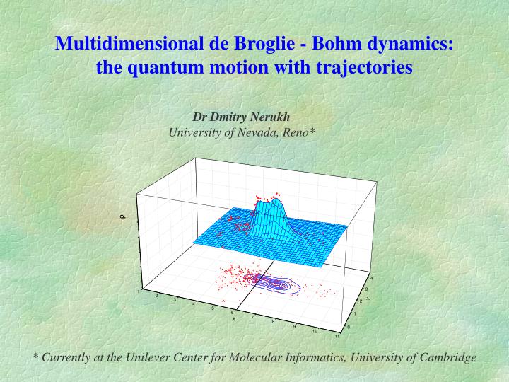
Multidimensional de Broglie - Bohm dynamics: the quantum motion with trajectories Dr Dmitry NerukhUniversity of Nevada, Reno* * Currently at the Unilever Center for Molecular Informatics, University of Cambridge
Prof. John H. Frederick Dr Clemens Woywod
de Broglie - Bohm interpretation of quantum mechanics Quantization particle wave position in space function observables: functions operators ‘Copenhagen interpretation’ of quantum mechanics Einstein point of view ‘statistical’ interpretation of wave function ‘Causal interpretation’ of quantum mechanics ‘pilot wave’: Louis de Broglie – 1927 Solvay Conference ‘quantum motion’: David Bohm – Phys. Rev., 85, 166-179, 180-193 (1952) Peter R. Holland, The quantum theory of motion, Cambridge University Press, 1993 http://www.netcomuk.co.uk/~jvpearce/bohm/bohm.html http://www.tiac.net./users/fbh
Hamilton-Jacobi theory Hamilton-Jacobi equation: where - the Hamilton principal function, single particle in external potential V: ,where Hamilton-Jacobi equation: The equation of motion:
the propagation of the S-function particle trajectory generalized Hamilton-Jacobi theory: particle dynamics evolution of the Sfield define S as a physical field find particle trajectories defines the particle trajectories; S has properties of a field Generalized Hamilton-Jacobi equation The equation of motion
Basic idea: quantum potential and quantum particles • The postulates of de Broglie-Bohm quantum theory of motion • a system comprises a wave propagating in space and time together with a particle which moves continuously under the guidance of the wave; • the wave is described by , a solution to the Schrödinger eq.; • the particle motion is the solution to the equation • where is a phase of ; the initial condition must be specified; the ensemble of the trajectories is generated by varying ; • the probability that a particle lies between andat time is given bywhere.
Reformulation of the Schrödinger equation Wavefunction in a polar form = Substituting into the time-dependent Schrödinger equation ‘Quantum’ potential: and separating real and imaginary parts: compare to
Example Simulation of a double slit experiment in two dimensions. The trajectories of an ensemble at the lower slit only are superposed on the interference pattern
Numerical Method Delaunay tesselation of the argument points and mapping the line along the derivative axis onto the tesselation structure. The points of intersection of the upper red line and edges of the triangles are used to approximate the cut of the surface
Scattering of 2D wavepacket from the Eckart barrier The potential: Eckart barrier (a.u.): Height Width Position 2D Eckart barrier – harmonic potential surface
time: 0 au Propagation of the Gaussian wavepacket on the Eckart barrier-harmonic potential surface • Simulation parameters: • · number of particles: 386 • · initial kinetic energy of the particles: 20 a.u. • · time step: 0.01 au • · total propagation time: 1.2 au • · calculation time: 0.5 hours (Pentium II, 400 MHz)
time: 108 au Propagation of the Gaussian wavepacket on the Eckart barrier-harmonic potential surface
time: 173 au Propagation of the Gaussian wavepacket on the Eckart barrier-harmonic potential surface
Scattering of 3D wavepacket from the Eckart barrier time: 0 au Propagation of the Gaussian wavepacket on 3D Eckart barrier-harmonic potential surface
time: 108 au Propagation of the Gaussian wavepacket on 3D Eckart barrier-harmonic potential surface
time: 173 au Propagation of the Gaussian wavepacket on 3D Eckart barrier-harmonic potential surface
Summary • It works • The calculation time increases slower then exponential with imensionality • Extremely well developed methods of propagating classical trajectories and constructing Delaunay tesselation • Easily visualizable • Natural introduction of various ‘mixed’ quantum-classical approaches