Download
1 / 93
930 likes | 1.18k Views
8-4: SHEAR STRESS DISRIBUTION IN FULLY DEVELOPED PIPE FLOW. rx = (r/2)(dp/dx) + c 1 /r FROM FORCE BALANCE c 1 = 0 or else rx becomes infinite rx = (r/2)(dp/dx) wall = (R/2)(dp/dx) HAVE NOT USED LAMINAR FLOW RELATION: rx = (du/dr)

E N D
8-4: SHEAR STRESS DISRIBUTION IN FULLY DEVELOPED PIPE FLOW rx = (r/2)(dp/dx) + c1/r FROM FORCE BALANCE c1 = 0 or else rx becomes infinite rx = (r/2)(dp/dx) wall = (R/2)(dp/dx) HAVE NOT USED LAMINAR FLOW RELATION: rx = (du/dr) rx = (r/2)(dp/dx) wall = (R/2)(dp/dx) TRUE FOR BOTH LAMINAR AND TURBULENT FLOW!!! Even though rx = (du/dr) + u’v’ in turbulent flow!!!
u’v’ DO NOT KNOW AS FUNCTION OF MEAN VELOCITY!!!!!!!! u’v’ modeled as duavg/dy and lm2(duavg/dy)2 but and lm vary from flow to flow and from place to place within a flow
-u’v’ = + if duavg/dy 0 u’v’ = 0 if duavg/dy = 0 Davies
Viscous Sublayer Viscous sublayer very thin: for 3”id pipe and uavg = 10 ft/sec, about 0.002” thick
rx = (du/dr) + u’v’ rx / = (du/dr) + u’v’ [rx / ]1/2 has units of velocity [wall / ]1/2 = u* (friction of shear stress velocity) u*~u’ near the wall Re = uavgD/ Re near wall = u*y/
u’v’ = 0 at the wall (no eddies) and at centerline (no mean velocity gradient) and approximately constant around r/R=0.1 u’v’/(u*)2 y+= yu*/ u* = [wall / ]1/2 u’v’/(u*)2 y/a Data from Laufer 1954
By a careful use of dimensional analysis in 1930 Prandtl deduced that near the wall: u = f(, wall, , y) u+ = u/u* = f(y+= yu*/) LAW OF THE WALL – inner layer
Near wall variables: y+ = yu*/ y = R-r u+ = u/u* u+/y+ = (u/u*)(/yu*) = u /(yu*u*) = (u /y)(wall/)-1 = (u/y)(wall)-1wall = du/drwall = u/y r R u+/y+ ~ 1 0y*5-7 viscosity dominates Viscous Sublayer
In 1937 C. B. Millikan showed that in the overlap layer the velocity must vary logarithmically with y: u/u* = (1/)ln(yu*/) + B Experiments show that: 0.41 and B0.5 u/u* = 2.5 ln(yu*/) + 5.0 LOGARITHMIC OVERLAP LAYER
For pipe at center: u/u* = 2.5 ln(yu*/) + 5.0 (a) Becomes: Uc/l/u* = 2.5 ln(Ru*/) + 5.0 (b) (b)-(a): (Uc/l-u)/u* = 2.5ln[(yu*/)/ (Ru*/)] (Uc/l-u)/u* = 2.5ln[y/R] Eq.(8-21) y = 0 no good!
Aside ~ Again using dimensional reasoning in 1933 Karman deduced that far from the wall: u = f(, wall, ) independent of viscosity, is boundary layer thickness (u=U for y > ) (U-u)/u* = g(y/) VELOCITY DEFECT LAW
u/u* = 2.5 ln(yu*/) + 5.0 Serendipitously, experiments show that the overlap layer extends throughout most of the velocity profile particularly for decreasing pressure gradients. The inner layer that is governed by the law of the wall typically is less than 2% of the velocity profile.
Pipe r=0 u+=y+ U*=2.5lny+ + 5 u+ = u/u* u+ = u/u* u+=y+ U*=2.5lny+ + 5
Empirically for smooth pipes it is found that the mean velocity profile can be expresses to a good approx. as: u(r)/Uc/l = (y/R)n = ([R-r]/R)1/n= (1-r/R)1/n n=6-10 Laminar Flow u/Uc/l = 1-(r/R)2 n = -1.7 + 1.8log(ReUcenterline) From experiment
u/Uc/l = (y/R)1/n = ([R-r]/R)1/n = (1-r/R)1/n Power law profile good near wall?
u/Uc/l = (y/R)1/n = ([R-r]/R)1/n = (1-r/R)1/n Power law profile deviates close to wall
u/Uc/l = (y/R)1/n = ([R-r]/R)1/n = (1-r/R)1/n Power law profile good at r = 0?
u/Uc/l = (y/R)1/n = ([R-r]/R)1/n = (1-r/R)1/n du/dy = Uc/l (1/n)R1/ny(1/n)-1 at y = 0 blows up Power Law profile no good at r = 0
TO PROVE: V/Uc/l = {2n2/(2n+1)(n+1)} Eq. (8.24) Fox et al. Strategy: find V = Q/A u/Uc/l = (y/R)1/nnote: u is a f(y), V is not a f(y) u /Uc/l = (y/R)n = ([R-r]/R)1/n= (1-r/R)1/n Q = 2ru(r)dr = 2rUc/l(y/R)1/ndr from 0-R y=R-r; r=0, y=R -dy=dr; r=R, y=0 Q=2rUc/l(y/R)1/ndr = 2(R-y)Uc/l(y/R)1/n(-dy) from R-0
TO PROVE: V/Uc/l = {2n2/(2n+1)(n+1)} Q=2rUc/l(y/R)1/ndr = 2(R-y)Uc/l(y/R)1/n(-dy) from R-0 = 2Uc/l{R(y/R)1/n(-dy) + (-y)(y/R)1/n(-dy)}from R-0 = 2Uc/l{R(y/R)1/n(dy) + (-y)(y/R)1/n(dy)} from 0-R = 2Uc/l{R1-1/ny1/n+1/(1+1/n) - R-1/ny1+1/n+1/(1+1/n +1)}|0R
TO PROVE: V/Uc/l = {2n2/(2n+1)(n+1)} Q: = 2Uc/l{R1-1/ny1/n+1/(1+1/n) - R-1/ny1+1/n+1/(1+1/n +1)}|0R = 2Uc/l{R2/(1+1/n) – R2/(2+1/n)} = 2Uc/l{nR2/(n+1) – nR2/(2n+1)} = 2Uc/l{(2n+1)nR2/(2n+1)(n+1)–(n+1)nR2/(n+1)(2n+1)}
TO PROVE: V/Uc/l = {2n2/(2n+1)(n+1)} Q: = 2Uc/l{(2n+1)nR2/(2n+1)(n+1)–(n+1)nR2/(n+1)(2n+1)} = 2Uc/l{nnR2/(2n+1)(n+1)} V = Q/R2= 2Uc/l{n2/(2n+1)(n+1)} V/Uc/l = uavg/uc/l = {2n2/(2n+1)(n+1)} Q.E.D.
With increasing n (Re) velocity gradient at wall becomes steeper, wall increases V/Uc/l = uavg/uc/l = 2n2/(n+1)(2n+1) = 2n2/(2n2+n+2n+1) = 2/(2+3/n +1/n2) As n , uavg /uc/l 1 For laminar flow uavg /uc/l = 1/2
CONSERVATION of ENERGY Chapter 4.8 rate of change of total energy of system = net rate of energy addition by heat transfer to fluid + net rate of energy addition by work done on fluid
CONSERVATION of ENERGY Chapter 4.8 Specific internal energy Total energy
Conservation of Energy EQ. 4.56: Total energy Internal energy only pressure work also steady, 1-D, incompressible
+ for going in + for going out • Wnormal = Fnormal ds • work done on area element • d Wnormal / dt = Fnormal V = p dA V • rate of work done on area element • - d Wnormal /dt = - p dA V = - p(v)dA V 1
0 0 0 0 If no heat (Q) transfer then: = 0 Mechanical energy
8-6: ENERGY CONSIDERATIONS IN PIPE FLOW ENERGY EQUATION (Eq. 4.56) dm/dt
Velocity not constant at sections 1 and 2. Need to introduce a correction factor, , that allows use of the average velocity, V, to compute kinetic energy at a cross section.
V = f(y) V f(y) LAMINAR FLOW: the kinetic energy coefficient, , = 2 (HW 8.66) FOR TURBULENT FLOW: the kinetic energy coefficient, (Re), 1 (HW 8.67) More specifically, = (Uc/l/V)3(2n2)/[(3+n)(3+2n)] n = 6, = 1.08; n=10, =1.03
Dividing by mass flow rate, dm/dt, gives: (Q/dt)/(dm/dt) = Q/dm
p/ + V2/2 + gz represents the mechanical energy per unit mass at a cross section (u2 –u1) - Q/dm = hlT represents the irreversible conversion of mechanical energy per unit mass to thermal energy , u2-u1, per unit mass and the loss of energy per unit mass, -Q/dm, via heat transfer
What are units of hlT ? What are units of HlT? Energy loss per unit mass of flowing fluid “one of the most important and useful equations in fluid dynamic” Fox et al. Energy loss per unit weight of flowing fluid
Units of hlT are L2/t2, If divide by g, get units of length for HlT Unfortunately both hlT and HLT are referred to as total total head loss. “one of the most important and useful equations in fluid dynamic” Energy loss per unit mass of flowing fluid Energy loss per unit weight of flowing fluid
Energy loss per unit mass of flowing fluid “one of the most important and useful equations in fluid dynamic” What provides energy input to match energy loss?
Energy loss per unit mass of flowing fluid “one of the most important and useful equations in fluid dynamic” Pumps, fans and blowers provide ppump/ = hpump (pump supplies pressure to overcome head loss, not K.E.) (power supplied by pump = Q ppump [m3t-1Fm-2 = Wt-1)
Convenient to break up energy losses, hlT, in fully developed pipe flow to major loses, hl, due to frictional effects along the pipe and minor losses, hlm, associated with entrances, fittings, changes in area,… For fully developed flow of constant pipe area: = 0 if pipe horizontal
LAMINAR FLOW: Calculation (THEORETICAL) of Head Loss Eq. 8.13c (p1 –p2)/ = p/ = hl (major head loss) Eq. (8.32) p = hl units of energy per unit mass. hl =p/ = (64/Re)(L/D)(uavg2/2); (p/L)D / (1/2 uavg2) = fD = 64/Re