Download
1 / 24
260 likes | 465 Views
Application of differential equations to model the motion of a paper helicopter. Kevin J. LaTourette Advisor Kris Green Spring 2007 Science Scholars Presentation St. John Fisher College. Outline. Helicopter Design (previous work) Rotational motion Helicopter drop Analytical solutions

E N D
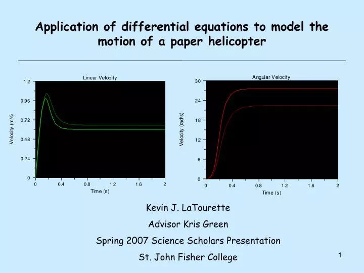
Application of differential equations to model the motion of a paper helicopter Kevin J. LaTourette Advisor Kris Green Spring 2007 Science Scholars Presentation St. John Fisher College
Outline • Helicopter Design (previous work) • Rotational motion • Helicopter drop • Analytical solutions • Future work
Helicopter design can greatly change the flight patterns of the helicopter • Wing length and width have large effects on rotational and linear velocities • Larger helicopters suffer from deformity due to strength of paper • Current model provides for the longest drop time • Same model used for all drops [1]
At equilibrium, the drag force deflects the rotors upward • Rotor deflection angle (wing flex), φ, decreases as linear velocity increases • At terminal linear velocity, φ ≈ 70˚ φ
Turbulence due to the wake of rotors was ignored • Wing blade has negligible thickness (100 μm) • Angular velocity is relatively low (ωT ≈ 20 rad/s) [4]
Due to rotation of the rotors, the drag force acts on a larger effective area • As the helicopter falls, it spins quickly, and the drag force acts on an area proportional to the circle traced by the wings as they rotate • Effective rotor area is a linear combination of the stationary wing area and the disc traced as the wings rotate
The rotational ‘blur’ effectively adds to the area the drag force acts on • This correction adds approximately 25% to the area of the rotors for small Δt [1]
Determination of angular velocity depended largely on the capabilities of the sensor • Our first experiment was designed to determine whether our data collection method was possible • Linear position was held constant, and rotor rotation was controlled • By obtaining a set of static rotational speeds, we could compare the results with the results of the actual drops
While the results were encouraging, it proved difficult to apply this technique to our drops
To reduce crosswinds and eliminate reflective noise, a large ‘box’ was constructed • At just over 3 meters tall, and 1 meter wide to account for the 15˚ arc swept out by the sensor • Only interested in the initial drop (1-2 seconds)
While the data gave good linear data, the angular resolution was poor • Data sensor operates at ~20 Hz, too low for credible angular rotation data analysis • If helicopter path is not directly lined up with sensor during the entire fall, we lose angular data • Chose not to use this technique for angular rotation • vt= 0.60 m/s ± 0.02 m/s
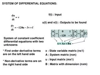
An understanding of the forces involved allow us to create differential equations
Incorrect assumption for bodies falling in Earth’s atmosphere Experimentally, the drag force has been approximated by [5] The resistance experienced by an object moving through a fluid is dependent on its velocity • Generally • b is constant, and depends on viscosity of the fluid, and the size and shape of the object • α depends on shape of object and size of the object • For small objects, • Raindrop falling in air • Aerosols falling in air • Objects passing through heavy oil
Applying this linearly, we obtain our linear drag force • Dependent on shape, b is not constant for our purposes • Incorporates effective rotor area A(ω, φ) • Also dependent on density of air [7] • We also introduce the coefficient of drag, cD • Surface/Shape of object • Viscosity of air (fluid)
We find the rotational drag force is dependent only on the angular velocity • Area of the helicopter does not change with increased linear or angular velocities, only wing deflection angle (assumed constant) • Recall v = rω • Torque
Our two coupled differential equations provide insight into the flight of the helicopter • Linear equation incorporates the summation of the falling body and the drag associated with the fall, which varies with both linear and angular velocities [1] • Angular equation experiences a forcing from the liner motion, and a separate drag force which varies only with the angular velocity • β and γ are scaling factors with units of length
With some careful rearrangement we arrive at our differential equations • Linear equation • v = linear velocity • ω = angular velocity • g = acceleration due to gravity (9.81m/s2) • m = mass of helicopter • Kv & Kvω= Linear drag force coefficients • Angular equation • β = linear drag scaling factor • I = moment of inertia • γ = angular drag scaling factor • Kω = angular drag force coefficients • K – equations • ρ = density of dry air • L = rotor length • W = rotor width • cD= coefficient of drag • r = rotor radius • Δt = change in time (~0.10 s)
Graphical solutions to our equations reflect the physical results • When dropped, the helicopter accelerates uniformly as there is no rotational motion • When the rotation begins, the linear velocity decreases, and the two settle into an equilibrium – the terminal velocities • vt= 0.62 m/s • vt experimental= 0.60 m/s ± 0.02 m/s • ωt= 21.49 rad/s • Numerical Solutions found using ODE Architect, implementing a fourth order Runge-Kutta Method
Analytical solutions to our system of equations provides insight into the terminal velocities • Obtained by setting • In turn, we can solve for β and γ in terms of the angular velocities, which we have determined experimentally
Our experimental determination of β and γprovide our final numerical solutions • vt= 0.60 m/s • vt (old)= 0.62 m/s • ωt=27.56 rad/s • ωt (old)= 21.49 rad/s • As expected, the terminal linear velocity is predicted exactly • Terminal angular velocity is higher than the previous prediction • No reliable data
Futures projects would be expected to obtain better experimental data • Other considerations include: • Accounting for the processional motion (wobble) about the z-axis as the helicopter falls • Incorporate a variable wing flex angle φ, which will provide a more accurate solution • Eliminate physical distortion by using a rigid model • Construct a better enclosure (Circular?) • Obtain better values for coefficient of drag and the scaling factors (β, γ)
Conclusion/Summary Application of differential equations to model the motion of a paper helicopter • Analytical solutions made significant improvements over previous models • Data collection was only successful for linear motion, but further measures must be taken for determining the angular motion • Sonic motion sensor may not be a possible data collection source • Several major assumptions were made for the sake of simplification, and would help us understand the motion much better • Future projects may wish to test different helicopter dimensions, to ensure the model is accurate
Acknowledgements • I would like to thank Dr. Kris Green for his assistance and helpful comments & the Mathematics Department, as well as Dr. Foek T. Hioe and the entire Physics department for ideas and suggestions and for the use of laboratories and supplies during the course of my research. • I also must express my great appreciation to Saint John Fisher College and the Science Scholars program for support and the opportunity to conduct research at the undergraduate level
References • Annis, D. (2005). Rethinking the Paper Helicopter: Combining Statistical and Engineering Knowledge. The American Statistician, 59, No. 4. (pp 320-326). • Fowles, G. & Cassiday, G. (2005). Analytical Mechanics, Seventh Edition. CA: Brooks/Cole. • Giancoli, D. (2000). Physics for Scientists & Engineers. Third Edition. NJ: Prentice Hall. • Iosilevskii, A., Isoilevskii, G. & Rosen, A. (1999). Asymptotic Aerodynamic Theory of Oscillating Rotary Wings in Axial Flight. SIAM Journal on Applied Mathematics, Vol. 59, No. 4. pp. 1371-1412. • Long, L. and Weiss, H. (1999). “The Velocity Dependence of Aerodynamic Drag: A Primer for Mathematics.” The American Mathematical Monthly. Vol 106, No. 2. p.127-135 • Nagle, R. & Staff, E. & Snider, A. (2004). Fundamentals of Differential Equations, Sixth Edition. NY: Pearson Education. • Weast, R. (1973). Handbook of Chemistry and Physics, 54th Edition. OH: Chemical Rubber Publishing Company.