Download
1 / 62
620 likes | 627 Views
Unit 4: Inferences about a Single Quantitative Predictor. Unit Organization. First consider details of simplest model (one parameter estimate; mean-only model; no X’s) Next examine simple regression (two parameter estimates, one X for one quantitative predictor variable)

E N D
Unit Organization • First consider details of simplest model (one parameter estimate; mean-only model; no X’s) • Next examine simple regression (two parameter estimates, one X for one quantitative predictor variable) • These provide critical foundation for all linear models • Subsequent units will generalize to one dichotomous predictor variable (Unit 5; Markus), multiple predictor variables (Units 6-7) and beyond….
Linear Models as Models • Linear models (including regression) are ‘models’ • DATA = MODEL + ERROR • Three general uses for models: • Describe and summarize DATA (Ys) in a simpler form using MODEL • Predict DATA (Ys) from MODEL • Will want to know precision of prediction. How big is error? Better prediction with less error. • Understand (test inferences about) complex relationships between individual regressors (Xs) in MODEL and the DATA (Ys). How precise are estimates of relationship? • MODELS are simplifications of reality. As such, there is ERROR. They also make assumptions that must be evaluated
Fear Potentiated Startle (FPS) • We are interested in producing anxiety in the laboratory • To do this, we develop a procedure where we expose people to periods of unpredictable electric shock administration alternating with periods of safety. • We measure their startle response in the shock and safe periods. • We use the difference between their startle during shock – safe to determine if they are anxious. • This is called Fear potentiated startle (FPS). Our procedure works if FPS > 0. We need a model of FPS scores to determine if FPS > 0.
Fear Potentiated Startle: One parameter model A very simple model for the population of FPS scores would predict the same value for everyone in the population. Yi = 0 We would like this value to be the “best” prediction. In the context of DATA = MODEL + ERROR, how can we quantify “best”? ^ We want to predict some characteristic about the population of FPS scores that minimizes the ERROR from our model. ERROR = DATA – MODEL i= Yi – Yi; There is an error (i) for each population score. How can we quantify total model error? ^
Total Error Sum of errors across all scores in the population isn’t ideal b/c positive and negative errors will tend to cancel each other (Yi – Yi) Sum of absolute value of errors could work. If we selected 0 to minimize the sum of the absolute value of errors, 0 would equal the median of the population. ( |Yi – Yi| ) Sum of squared errors (SSE) could work. If we selected 0 to minimize the sum of squared errors, 0 would equal the mean of the population. ^ ^ ^ (Yi – Yi)2
One parameter model for FPS For the moment, lets assume we prefer to minimize SSE (more on that in a moment). You should predict the population mean FPS for everyone. Yi = 0where 0= What is the problem with this model and how can we fix this problem? ^ We don’t know the population mean for FPS scores (). We can collect a sample from the population and use the sample mean (X) as an estimate of the population mean (). X is an unbiased estimate for
Model Parameter Estimation Population model Yi = 0where 0= Yi = 0 + i Estimate population parameters from sample Yi = b0where b0 = X Yi = b0 + ei ^ ^
Least Squares Criterion In ordinary least squares (OLS) regression and other least squares linear models, the model parameter estimates (e.g., b0) are calculated such that they minimize the sum of squared errors (SSE) in the sample in which you estimate the model. SSE = (Yi – Yi)2 SSE = ei2 ^
Properties of Parameter Estimates There are 3 properties that make a parameter estimate attractive. Unbiased: Mean of the sampling distribution for the parameter is equal to the value for that parameter in the population. Efficient: The sample estimates are close to the population parameter. In other words, the narrower the sampling distribution for any specific sample size N, the more efficient the estimator. Efficient means small SE for parameter estimate Consistent: As the sample size increases, the sampling distribution becomes narrower (more efficient). Consistent means as N increases, SE for parameter estimate decreases
Least Squares Criterion If the i are normally distributed, both the median and the mean are unbiased and consistent estimators. The variance of the sampling distribution for the mean is: 2 N The variance of the sampling distribution for the median is: 2 2N Therefore the mean is the more efficient parameter estimate. For this reason, we tend to prefer to estimate our models by minimizing the sum of squared errors.
Fear-potentiated startle during Threat of Shock > setwd("C:/Users/LocalUser/Desktop/GLM") > d = lm.readDat('4_SingleQuantitative_FPS.dat') > str(d) 'data.frame': 96 obs. of 2 variables: $ BAC: num 0 0 0 0 0 0 0 0 0 0 ... $ FPS: num -98.098 -22.529 0.463 1.194 2.728 ... > head(d) BAC FPS 0125 0 -98.0977778 0013 0 -22.5285000 0113 0 0.4632944 0116 0 1.1943667 0111 0 2.7280444 0014 0 6.7237833 > some(d) BAC FPS 0111 0.0000 2.728044 1121 0.0235 43.901667 1126 0.0395 14.181344 1113 0.0495 53.176722 1124 0.0580 11.859050 1112 0.0605 45.181778 2112 0.0730 162.736611 2016 0.0750 30.453111 2023 0.0925 19.598722 3112 0.1085 14.603611
Descriptives and Univariate Plots > lm.describeData(d) var n mean sd median min max skew kurtosis BAC 1 96 0.06 0.04 0.06 0.0 0.14 -0.09 -1.09 FPS 2 96 32.19 37.54 19.46 -98.1 162.74 0.62 1.93 > windows() #on MAC, use quartz() > par('cex' = 1.5, 'lwd'=2) > hist(d$FPS)
FPS Experiment: The Inference Details • Goal: Determine if our shock threat procedure is effective at potentiating startle (increasing startle during threat relative to safe) • Create a simple model of FPS scores in the population • FPS = 0 • Collect sample of N=96 to estimate 0 • Calculate sample parameter estimate (b0) that minimizes SSE in sample • Use b0 to test hypotheses • H0: 0 = 0 • Ha: 0 <> 0
Estimating a one parameter model in R m = lm(FPS ~ 1, data = d) > summary(m) Call: lm(formula = FPS ~ 1, data = d) Residuals: Min 1Q Median 3Q Max -130.29 -25.40 -12.73 18.27 130.55 Coefficients: Estimate Std. Error t value Pr(>|t|) (Intercept) 32.191 3.832 8.402 4.26e-13 *** --- Signif. codes: 0 ‘***’ 0.001 ‘**’ 0.01 ‘*’ 0.05 ‘.’ 0.1 ‘ ’ 1 Residual standard error: 37.54 on 95 degrees of freedom
Errors/Residuals summary(m) Call: lm(formula = FPS ~ 1, data = d) Residuals: Min 1Q Median 3Q Max -130.29 -25.40 -12.73 18.27 130.55 Coefficients: Estimate Std. Error t value Pr(>|t|) (Intercept) 32.191 3.832 8.402 4.26e-13 *** --- Signif. codes: 0 ‘***’ 0.001 ‘**’ 0.01 ‘*’ 0.05 ‘.’ 0.1 ‘ ’ 1 Residual standard error: 37.54 on 95 degrees of freedom This is simple descriptive information about the errors (ei) ei = (Yi – Yi) ^
Errors/Residuals ^ ei = (Yi – Yi) R can report errors for each individual in the sample: > residuals(m) 0125 0013 0113 0116 0111 0014 0124 0022 -130.2886183 -54.7193405 -31.7275460 -30.9964738 -29.4627960 -25.4670572 -25.3710072 -16.8541238 0011 0021 0121 0016 0123 0122 0012 0115 -12.6999127 -2.7175738 1.5669373 8.3829373 9.3662151 11.7176040 16.2161040 19.1260706 0023 0026 0114 0126 0015 0024 0112 0025 19.6643817 35.0963817 36.5672151 53.1913817 57.4678817 58.6873817 72.7258928 78.7543262 1121 1014 1122 1025 1023 1126 1125 1011 11.7108262 34.7095484 -25.2434516 14.2658262 104.6339928 -18.0094960 -8.4337683 29.8681317 1115 1021 1116 1013 1024 1111 1113 1012 -24.1598966 61.4058262 -19.2076849 -14.1219516 36.5526595 -29.6592294 20.9858817 59.8164373 2014 1114 1022 1123 1026 1016 3025 1124 -35.5108960 -29.1695572 67.7537262 -18.4250627 -16.7506349 47.3338484 -21.4997294 -20.3317905 2122 1112 2011 2013 2022 1015 2124 2024 27.5951151 12.9909373 -12.7704849 -58.2597294 -35.5405016 17.9774928 -28.5735072 25.0772151 2113 2116 2112 3024 2025 2123 2016 2015 5.2138262 -27.4784549 130.5457706 1.6943262 -20.6439405 -28.0089794 -1.7377294 -32.0183927 2125 2111 2126 2026 2121 2012 2115 3015 -23.4260627 9.3974373 4.5087151 37.4066428 17.0578817 3.9210484 -9.8150183 27.4325484 3023 2114 2021 3026 2023 3116 3121 3013 -14.5139683 -13.0036627 0.3123817 -25.3833322 -12.5921183 -32.1845627 -31.0086183 -18.5716738 3022 3021 3014 3125 3011 3122 3114 3016 6.1488262 -18.1054016 -17.1700072 -31.8114616 77.8639373 -34.0540127 4.8073817 -26.4386960 3112 3115 3111 3124 3126 3113 3012 3123 -17.5872294 -26.9565572 -26.9358794 -31.4756127 -15.9328183 -25.7722738 -21.4575572 -17.4630572 You can get the SSE easily: > sum(residuals(m)^2) [1] 133888.3
Standard Error of Estimate summary(m) Call: lm(formula = FPS ~ 1, data = d) Residuals: Min 1Q Median 3Q Max -130.29 -25.40 -12.73 18.27 130.55 Coefficients: Estimate Std. Error t value Pr(>|t|) (Intercept) 32.191 3.832 8.402 4.26e-13 *** --- Signif. codes: 0 ‘***’ 0.001 ‘**’ 0.01 ‘*’ 0.05 ‘.’ 0.1 ‘ ’ 1 Residual standard error: 37.54 on 95 degrees of freedom This is the standard error of estimate. It an estimate of the standard deviation of i (Yi – Yi)2SSE N - P N - P NOTE: for mean-only model, this is sY ^
Coefficients (Parameter Estimates) summary(m) Call: lm(formula = FPS ~ 1, data = d) Residuals: Min 1Q Median 3Q Max -130.29 -25.40 -12.73 18.27 130.55 Coefficients: Estimate Std. Error t value Pr(>|t|) (Intercept) 32.191 3.832 8.402 4.26e-13 *** --- Signif. codes: 0 ‘***’ 0.001 ‘**’ 0.01 ‘*’ 0.05 ‘.’ 0.1 ‘ ’ 1 Residual standard error: 37.54 on 95 degrees of freedom This is b0, the unbiased sample estimate of 0, and its standard error. It is also called the intercept in regression (more on this later). Yi = b0 Yi = 32.2 > coef(m) (Intercept) 32.19084 ^ ^
Predicted Values ^ Yi = 32.19 You can get the predicted value for each individual in the sample using this model: > fitted.values(m) 0125 0013 0113 0116 0111 0014 0124 0022 0011 0021 0121 0016 32.19084 32.19084 32.19084 32.19084 32.19084 32.19084 32.19084 32.19084 32.19084 32.19084 32.19084 32.19084 0123 0122 0012 0115 0023 0026 0114 0126 0015 0024 0112 0025 32.19084 32.19084 32.19084 32.19084 32.19084 32.19084 32.19084 32.19084 32.19084 32.19084 32.19084 32.19084 1121 1014 1122 1025 1023 1126 1125 1011 1115 1021 1116 1013 32.19084 32.19084 32.19084 32.19084 32.19084 32.19084 32.19084 32.19084 32.19084 32.19084 32.19084 32.19084 1024 1111 1113 1012 2014 1114 1022 1123 1026 1016 3025 1124 32.19084 32.19084 32.19084 32.19084 32.19084 32.19084 32.19084 32.19084 32.19084 32.19084 32.19084 32.19084 2122 1112 2011 2013 2022 1015 2124 2024 2113 2116 2112 3024 32.19084 32.19084 32.19084 32.19084 32.19084 32.19084 32.19084 32.19084 32.19084 32.19084 32.19084 32.19084 2025 2123 2016 2015 2125 2111 2126 2026 2121 2012 2115 3015 32.19084 32.19084 32.19084 32.19084 32.19084 32.19084 32.19084 32.19084 32.19084 32.19084 32.19084 32.19084 3023 2114 2021 3026 2023 3116 3121 3013 3022 3021 3014 3125 32.19084 32.19084 32.19084 32.19084 32.19084 32.19084 32.19084 32.19084 32.19084 32.19084 32.19084 32.19084 3011 3122 3114 3016 3112 3115 3111 3124 3126 3113 3012 3123 32.19084 32.19084 32.19084 32.19084 32.19084 32.19084 32.19084 32.19084 32.19084 32.19084 32.19084 32.19084
Testing Inferences about 0 summary(m) Call: lm(formula = FPS ~ 1, data = d) Residuals: Min 1Q Median 3Q Max -130.29 -25.40 -12.73 18.27 130.55 Coefficients: Estimate Std. Error t value Pr(>|t|) (Intercept) 32.191 3.832 8.402 4.26e-13 *** --- Signif. codes: 0 ‘***’ 0.001 ‘**’ 0.01 ‘*’ 0.05 ‘.’ 0.1 ‘ ’ 1 Residual standard error: 37.54 on 95 degrees of freedom This is the t-statistic to test the H0 that 0 = 0. The probability (p-value) of obtaining a sample b0 = 32.2 if H0 is true (0 = 0) < .0001. Describe the logic of how this was determined?
Sampling Distribution: Testing Inferences about 0 H0: 0 = 0; Ha: 0 <> 0 If H0 is true, the sampling distribution for 0 will have a mean of 0. We can estimate standard deviation of the sampling distribution with SE for b0. t (df=N-P) = b0 – 0 = 32.2 – 0 = 8.40 SEb0 3.8 b0 is approximately 8 standard deviations above the expected mean of the distribution if H0 is true pt(8.40,95,lower.tail=FALSE) * 2 [1] 4.293253e-13 The probability of obtaining a sample b0 = 32.2 if H0 is true is very low (< .05). Therefore we reject H0 And conclude that 0 <> 0 and b0 is our best (unbiased) estimate of it.
Statistical Inference and Model Comparisons • Statistical inference about parameters is fundamentally about model comparisons • You are implicitly (t-test of parameter estimate) or explicitly (F-test of model comparison) comparing two different models of your data • We follow Judd et al and call these two models the compact model and the augmented model. • The compact model will represent reality as the null hypothesis predicts. The augmented model will represent reality as the alternative hypothesis predicts. • The compact model is simpler (fewer parameters) than the augmented model. It is also nested in the augmented model (i.e. a subset of parameters)
Model Comparisons: Testing inferences about 0 ^ • FPSi = 0 • H0: 0 = 0 • Ha: 0 <> 0 • Compact model: FPSi = 0; • Augmented model: FPSi = 0 ( b0) • We estimate 0 parameters (P=0) in this compact model • We estimate 1 parameter (P=1) in this augmented model • Choosing between these two models is equivalent to testing if 0 = 0 as you did with the t-test ^ ^
Model Comparisons: Testing inferences about 0 ^ • Compact model: FPSi = 0 • Augmented model: FPSi = 0 ( b0) • We can compare (and choose between) these two models by comparing their total error (SSE) in our sample • SSE = (Yi – Yi)2 • SSE(C) = (Yi – Yi)2 = (Yi – 0)2 • > sum((d$FPS - 0)^2) • [1] 233368.3 • SSE(A) = (Yi – Yi)2 = (Yi – 32.19)2 • > sum((d$FPS – coef(m)[1])^2 #(sum(residuals(m)^2) • [1] 133888.3 ^ ^ ^
Model Comparisons: Testing inferences about 0 ^ Compact model: FPSi = 0; SSE = 233,368.3 P = 0 Augmented model: FPSi = 0 ( b0) SSE = 133,888.3 P=1 F (PA – PC, N – PA) = (SSE(C) -SSE(A)) / (PA-PC) SSE(A) / (N-PA) F (1– 0, 96 – 1) = (233368.3-133888.3) / (1 - 0) 133888.3 / (96 - 1) F(1,95) = 70.59, p < .0001 > pf(70.58573,1,95, lower.tail=FALSE) [1] 4.261256e-13 ^
Effect Sizes • Your parameter estimates are descriptive. The describe effects in the original units of the (IVs) and DV. Report them in your paper • There are many other effect size estimates available. You will learn two that prefer. • Partial eta2 (p2): Judd et al call this PRE (proportional reduction in error) • Eta2 (2): This is also commonly referred to as R2 in regression.
Sampling Distribution vs. Model Comparison The two approaches to testing H0 about parameters (0, j) are statistically equivalent They are complementary approaches with respect to conceptual understanding of GLMs Sampling distribution Focus on population parameters and their estimates Tight connection to sampling and probability distributions Understanding of SE (sampling error/power; confidence intervals; graphic displays) Model comparison Focus on models themselves increase Highlights model fit (SSE) and model parsimony (P) Clearer link to PRE (p2) Test comparisons that differ by > 1 parameter (discouraged)
Partial Eta2 or PRE ^ Compact model: FPSi = 0; SSE = 233,368.3 P = 0 Augmented model: FPSi = 0 ( b0) SSE = 133,888.3 P=1 How much was the error reduced in the augmented model relative to the compact model? SSE(C) – SSE(A) = 233,368.3 - 133,888.3 = .426 SSE (C) 233,368.3 Our more complex model that includes 0reduces prediction error (SSE) by approximately 43%. Not bad! ^
Confidence Interval for b0 A confidence interval (CI) is an interval for a parameter estimate in which you can be fairly confident that you will capture the true population parameter (in this case, 0). Most commonly reported is the 95% CI. Across repeated samples, 95% of the calculated CIs will include the population parameter*. > confint(m) 2.5 % 97.5 % (Intercept) 24.58426 39.79742 Given what you now know about confidence intervals and sampling distributions, what should the formula be? CI (b0) = b0+ t (; N-P) * SEb0 For the 95% confidence interval this is approximately + 2 SEs around our unbiased estimate of 0
Confidence Interval for b0 How can we tell if a parameter is “significant” from the confidence interval? If a parameter <> 0 at = .05, then the 95% confidence interval for its parameter estimate should not include 0. This is also true for testing whether the parameter is equal to any other True for any other non-zero point estimate for the parameter non-zero value
The one parameter (mean-only) model: Special Case What special case (specific analytic test) is statistically equivalent to the test of the null hypothesis: 0 = 0 in the one parameter model? The one sample t-test testing if a population mean = 0. > t.test(d$FPS) One Sample t-test data: d$FPS t = 8.4015, df = 95, p-value = 4.261e-13 alternative hypothesis: true mean is not equal to 0 95 percent confidence interval: 24.58426 39.79742 sample estimates: mean of x 32.19084
Testing 0= non-zero values How could you test an H0 regarding 0 = some value other than 0 (e.g., 10)? HINT: There are at least three methods. ^ ^ Option 1: Compare SSE for the augmented model (Yi= 0 ) to SSE from a different compact model for this new H0 (Yi= 10) Option 2: Recalculate t-statistic using this new H0. t = b0 – 10 SEb0 Option 3: Does the confidence interval for the parameter estimate contain this other value? No p-value provided. > confint(m) 2.5 % 97.5 % (Intercept) 24.58426 39.79742
Intermission….. • One parameter (0) “mean-only” model • Description: b0 describes mean of Y • Prediction: b0 is predicted value that minimizes sample SSE • Inference: Use b0 to test if 0 = 0 (default) or any other value. One sample t-test. • Two parameter (0, 1) model • Description: b1 describes how Y changes as function of X1. b0 describes expected value of Y at specific value (0) for X1. Prediction: b0 and b1 yield predicted values that vary by X1 and minimize SSE in sample. • Inference: Test if 1 = 0. Pearson’s r; independent sample t-test. Test if 0 = 0. Analogous to one-sample t-test controlling for X1, if X1 is mean-centered. Very flexible!
Two Parameter (One Predictor) models We started with a very simple model of FPS: FPS = 0 What if some participants were drunk and we knew their blood alcohol concentrations (BAC). Would it help? What would the model look like? What question (s) does this model allow us to test? Think about it
The Two Parameter Model DATA = MODEL + ERROR Yi = 0 + 1 * X1 + i Yi = 0 + 1 * X1 i = Yi - Yi FPSi = 0 + 1 * BAC1 ^ ^ ^
The Two Parameter Model ^ Yi = 0 + 1 * X1 As before, the population parameters in the model (0 , 1) are estimated by b0 & b1 calculated from sample data based on the least squares criterion such that they minimize SSE in the sample data. Sample model Yi = b0 + b1 * X1 ^ To derive these parameter estimates you must solve series of simultaneous equations using linear algebra and matrices (see supplemental reading). Or use R!
Least Squares Criterion ^ ei = Yi – Yi SSE = ei2
Interpretation of b0 in Two Parameter Model ^ Yi = b0 + b1 * X1 b0is predicted value for Y when X1 = 0. Graphically, this is the Y intercept for the regression line (Value of Y where regression line crosses Y-axis at X1 = 0*). Approximately what is b0 in this example? 42.5
Interpretation of b0 in Two Parameter Model IMPORTANT: Notice that b0 is very different (42.5) in the two parameter model than in previous one parameter model (32.2) WHY? In the one parameter model b0 was our sample estimate of the mean FPS score in everyone. b0 in the two parameter model is our sample estimate of the mean FPS score for people with BAC = 0, not everyone.
Interpretation of b1 in Two Parameter Model ^ Yi = b0 + b1 * X1 b1is the predicted change in Y for every one unit change in X1. Graphically it is represented by the slope of the line regression line. If you understand the units of your predictor and DV, this is an attractive description of their relationship. ^ FPSi = 42.5 + -184.1 * BACi For every 1% increase in BAC, FPS decreases by 184.1 microvolts. For every .01% increase in BAC, FPS decreases by 1.841 microvolts.
Testing Inferences about 1 • Does alcohol affect people’s anxiety? • FPSi = 0 + 1 * BACi • What are your null and alternative hypotheses about model parameter to evaluate this question? ^ H0: 1 = 0 Ha: 1 <> 0 If 1 = 0, this means that FPS does not change with changes in BAC. In other words, there is no effect of BAC on FPS. If 1 < 0, this means that FPS decreases with increasing BAC (People are less anxious when drunk) If 1 > 0, this means FPS increases with increasing BAC (i.e., people are more anxious when drunk).
Estimating a Two Parameter Model in R > m2 = lm(FPS ~ BAC, data = d) > summary(m2) Call: lm(formula = FPS ~ BAC, data = d) Residuals: Min 1Q Median 3Q Max -140.555 -21.565 -8.289 15.638 133.718 Coefficients: Estimate Std. Error t value Pr(>|t|) (Intercept) 42.457 6.548 6.484 4.11e-09 *** BAC -184.092 95.894 -1.920 0.0579 . --- Signif. codes: 0 ‘***’ 0.001 ‘**’ 0.01 ‘*’ 0.05 ‘.’ 0.1 ‘ ’ 1 Residual standard error: 37.02 on 94 degrees of freedom Multiple R-squared: 0.03773, Adjusted R-squared: 0.02749 F-statistic: 3.685 on 1 and 94 DF, p-value: 0.05792
Testing Inferences about 1 Coefficients: Estimate Std. Error t value Pr(>|t|) (Intercept) 42.457 6.548 6.484 4.11e-09 *** BAC -184.092 95.894 -1.920 0.0579 . • Does BAC affect FPS? Explain this conclusion in terms of the parameter estimate, b1 and its standard error Under the H0: 1 = 0, the sampling distribution for 1 will have a mean of 0 with an estimated standard deviation of 95.894. t (96-1) = -184.092 – 0 = -1.92 95.894 Our this value of the parameter estimate, b1, is 1.92 standard deviations below the expected mean of the sampling distribution for H0. > pt(-1.92, 94, lower.tail = TRUE)*2 [1] 0.05788984 A b1 of this size is not unlikely under the null, therefore you fail to reject the null and conclude that BAC has no effect on FPS
Testing Inferences about 1 Coefficients: Estimate Std. Error t value Pr(>|t|) (Intercept) 42.457 6.548 6.484 4.11e-09 *** BAC -184.092 95.894 -1.920 0.0579 . One tailed p-value > pt(-1.92, 94, lower.tail = TRUE) [1] 0.02894492 Two-tailed p-value > pt(-1.92, 94, lower.tail = TRUE)*2 [1] 0.05788984 H0: 1 = 0 Ha: 1 <> 0
Model Comparison: Testing Inferences about 1 • H0: 1 = 0 • Ha: 1 <> 0 • What two models are you comparing when you test hypotheses about 1? Describe the logic. ^ Compact Model: FPSi = 0 + 0 * BACi PC = 1 SSE(C) = 133888.3 Augmented Model: FPSi = 0 + 1 * BACi PA = 2 SSE(A) = 128837.1 F(PA-PC, N-PA) = SSE(C) – SSE(A) / (PA-PC) SSE(A) / (N-PA) F(1,94) = 3.685383, p = 0.05792374 ^
Sum of Squared Errors If there is a perfect relationship between X1 and Y in your sample, what will the SSE be in the two parameter model and why? SSE(A) = 0 . All data points will fall perfectly on the regression line. All errors will be 0 If there is no relationship at all between X1 and Y in your sample (b1 = 0), what will the SSE be in the two parameter model and why? SSE(A) = SSE of the mean-only model. X1 provides no additional information about the DV. Your best prediction will still be the mean of the DV.
Testing Inferences about 0 Coefficients: Estimate Std. Error t value Pr(>|t|) (Intercept) 42.457 6.548 6.484 4.11e-09 *** BAC -184.092 95.894 -1.920 0.0579 . • What is the interpretation of b0 in this two parameter model? It is the predicted FPS for a person with BAC = 0 (sober). The test of this parameter estimate could inform us if the shock procedure worked among our sober participants. This is probably a more appropriate manipulation check than testing if it worked in everyone including drunk people given that alcohol could have reduced FPS. What two models are being compared? ^ Compact Model: FPSi = 0+ 1 * BACi Augmented Model: FPSi = 0+ 1 * BACi ^
Confidence Interval for bj or b0 You can provide confidence intervals for each parameter estimate in your model. > confint(m2) 2.5 % 97.5 % (Intercept) 29.45597 55.457721 BAC -374.49261 6.308724 The underlying logic from your understanding of sampling distributions remains the same CI (b) = b+ t (;N-P) * SEbwhere P = total # of parameters How can we tell if a parameter is “significant” from the confidence interval? If a parameter is <> 0, at = .05, then the 95% confidence interval should not include 0. True for any other non-zero value for b as well.
Partial Eta2 or PRE for 1 How can you calculate the effect size estimate partial eta2 (PRE) for 1 Compare the SSE across the two relevant models Compact Model: FPSi = 0 + 0 * BACi SSE(C) = 133888.3 Augmented Model: FPSi = 0 + 1 * BACi SSE(A) = 128837.1 SSE(C) – SSE(A) = 133888.3 - 128837.1 = . 0.038 SSE (C) 133888.3 Our augmented model that includes a non-zero effect for BAC reduces prediction error (SSE) by only 3.8% over the compact model that fixes this parameter at 0. ^ ^