Download
1 / 7
70 likes | 228 Views
Background Information. I. Measures of Return and Risk . A . Operational defn of Ex Post, Nominal Return . r = (ending value – beginning value + cash flows) / (beginning value) = (ending – beginning)/(beginning) + ( cash flows ) / ( beginning)

E N D
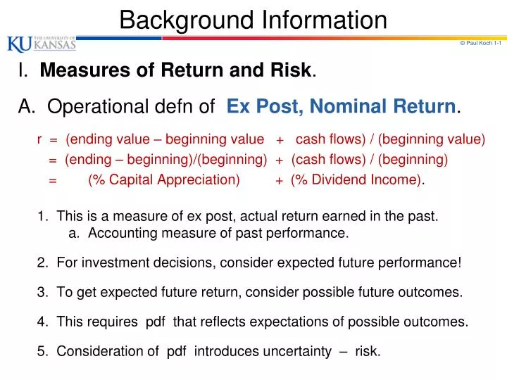
Background Information I. Measures of Return and Risk. A. Operational defnof Ex Post, NominalReturn. r = (ending value – beginning value + cash flows) / (beginning value) = (ending – beginning)/(beginning) + (cash flows) / (beginning) = (% Capital Appreciation) + (% Dividend Income). 1. This is a measure of ex post, actual return earned in the past. a. Accounting measure of past performance. 2. For investment decisions, consider expected future performance! 3. To get expected future return, consider possible future outcomes. 4. This requires pdfthat reflects expectations of possible outcomes. 5. Consideration of pdf introduces uncertainty – risk.
Background Information B. Ex Ante, Expected Return and Uncertainty. 1. Reflected in investor’s probability distribution function (pdf). 2. Consider the pdf’sof two possible investments, #1 & #2 : Investment: | #1 | #2 . Possible return (ri) | 6%| 2% 6% 10% Probability (pi) | 1.0 | 0.2 0.6 0.2 pi pi 1.0 | Investment #1 * 1.0 | | * | Investment #2 0.8 | * 0.8 | | * | 0.6 | * 0.6 | * | * | * 0.4 | * 0.4 | * | * | * 0.2 | * 0.2 | * * * |* .ri | * * * .ri 0 2% 6% 10% 0 2% 6% 10% 3. Investment #1 is a T.Bill; r = 6% with certainty (no risk). Investment #2 depends on future states of the world; uncertainty!
Background Information pi pi 1.0 | Investment #1 * 1.0 | | * | Investment #2 0.8 | * 0.8 | | * | 0.6 | * 0.6 | * | * | * 0.4 | * 0.4 | * | * | * 0.2 | * 0.2 | * * * |* .ri | * * * .ri 0 2% 6% 10% 0 2% 6% 10% 4. Expected Return = E( ri)= piri; i indexes states of world. a. For investment A, E( ri) = (1.0)(6%) = 6% b. For investment B, E( ri) = (.2)(2%) + (.6)(6%) + (.2)(10%) = 6% 5. Observe, expected return is the same for 1 & 2, but 2 has more risk. 6. In reality, pdf is continuous over (-,+); smooth bell-shaped curve. 7. For continuous pdf’s, E(ri) = ∫ f( ri) ridri; analogous to piri. -
Background Information C. How do we measure Risk? Variance = 2 = E[ ri - E(ri) ]2= pi [ri- E(ri)]2 . 1. For #1, 2 = (1.0)(.06 - .06)2 = 0. No uncertainty, no risk. 2. For #2, 2 = (.2)(.02-.06)2 + (.6)(.06-.06)2 + (.2)(.10-.06)2 = .00032 + 0 + .00032 = .00064 3. Standard Deviation, . For #1, = 0; For #2, .0253 4. For continuous case, 2 = ∫ f( ri) [ ri- E(ri) ]2 dri. 5. If ri deviates further from mean, distribution more spread out: [ ri- E(ri) ] is larger; [ ri- E(ri) ]2 is larger; 2 is larger.
Background Information D. Covariance. 1. Defn: 12= Cov(r1, r2) = E[r1 - E(r1)][r2 - E(r2)] n 2. Operational Defn: 12= (1/n) [r1i - E(r1)][r2i - E(r2)] i=1 3. Case i: Suppose most points, (r1i , r2i), are in 1st & 3rd quadrants. r2-E(r2) First quad: [r1 - E(r1)] > 0 |. . . [r2 - E(r2)] > 0 | . . . 12 > 0 . | . . . . __________ | _________ r1-E(r1) Third quad: [r1 - E(r1)] < 0 . . | . . [r2 - E(r2)] < 0 . . . . . | 12 > 0 .. . | |
Background Information 4. Case ii : Suppose most points, (r1i , r2i), are in 2nd & 4th quadrants. Second quad: [r1 - E(r1)] < 0 . r2-E(r2) [r2 - E(r2)] > 0 . . . . | 12 < 0 . . . . . | . __________ | _________ r1-E(r1) Fourth quad: [r1 - E(r1)] > 0 . . | . . . . [r2 - E(r2)] < 0 | . . . . 12 < 0 | . . • Case iii : Suppose points, (r1i , r2i), are scattered in all 4 quadrants. . r2-E(r2) . . Terms in 1st & 3rd quad → 12 > 0 . . . . | . . . . Terms in 2nd& 4th quad → 12 < 0 . . . . . | . . . . __________ | _________ r1-E(r1) Altogether, terms cancel out, . . . . . | . . . . so that 12 ≈ 0. . . . . | . . . . . . . | . . Point: Sign of 12 shows the nature of the relation between r1 & r2 , but not the strength of the relation.
Background Information E. Correlation = 12= 12 / 1 2 . 1. Note: 12 may vary between - & +. a. If r1 and/or r2 vary more widely (if 1 and/or 2 larger), then [r1 - E(r1)] and/or [r2 - E(r2)] are larger in magnitude, and 12 will be larger in mag. (depending on case i, ii, or iii). 2. Thus, magnitude of 12does not tell us about strength of relation. 3. Correlation fixes this problem; adjusts 12 for size of 1 and 2. a. If 12 is larger (because 1 and/or 2 larger), 12corrects for this by dividing 12 by (1 2). 4. Result: 12 varies between -1 and +1. a. If 12= +1, r1& r2 are perfectly positively related. b. If 12= -1, r1& r2 are perfectly negatively related. c. If 12= 0, r1& r2 are unrelated.