Download
1 / 60
630 likes | 824 Views
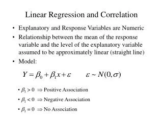
Linear Regression and Correlation. Fitted Regression Line. Equation of the Regression Line. Least squares regression line of Y on X. Regression Calculations. Plotting the regression line. Residuals. Using the fitted line, it is possible to obtain an estimate of the y coordinate.

E N D
Equation of the Regression Line Least squares regression line of Y on X
Residuals • Using the fitted line, it is possible to obtain an estimate of the y coordinate • The “errror” in the fit we term the “residual error”
Other ways to evaluate residuals • Lag plots, plot residuals vs. time delay of residuals…looks for temporal structure. • Look for skew in residuals • Kurtosis in residuals – error not distributed “normally”.
Model Residuals: constrained Model Residuals: freely moving Pairwise model Pairwise model Independent model Independent model -0.3 0 0.3 -0.3 0 0.3 Pairwise model Pairwise model Independent model Independent model
Parametric Interpretation of regression: linear models • Conditional Populations and Conditional Distributions • A conditional population of Y values associated with a fixed, or given, value of X. • A conditional distribution is the distribution of values within the conditional population above Population mean Y value for a given X Population SD of Y value for a given X
The linear model • Assumptions: • Linearity • Constant standard deviation
estimates estimates estimates Statistical inference concerning • You can make statistical inference on model parameters themselves
Standard error of slope • 95% Confidence interval for where
Hypothesis testing: is the slope significantly different from zero? = 0 Using the test statistic: df=n-2
Coefficient of Determination • r2, or Coefficient of determination: how much of the variance in data is accounted for by the linear model.
Correlation Coefficient • R is symmetrical under exchange of x and y.
What’s this? It adjusts R to compensate for the fact That adding even uncorrelated variables to the regression improves R
Statistical inference on correlations • Like the slope, one can define a t-statistic for correlation coefficients:
STA example • R2=0.25. • Is this correlation significant? • N=446, t = 0.25*(sqrt(445/(1-0.25^2))) = 5.45
When is Linear Regression Inadequate? • Curvilinearity • Outliers • Influential points
Outliers • Can reduce correlations and unduly influence the regression line • You can “throw out” some clear outliers • A variety of tests to use. Example? Grubb’s test • Look up critical Z value in a table • Is your z value larger? • Difference is significant and data can be discarded.
Influential points • Points that have a lot of influence on regressed model • Not really an outlier, as residual is small.
Conditions for inference • Design conditions • Random subsampling model: for each x observed, y is viewed as randomly chosen from distribution of Y values for that X • Bivariate random sampling: each observed (x,y) pair must be independent of the others. Experimental structure must not include pairing, blocking, or an internal hierarchy. • Conditions on parameters is not a function of X • Conditions concerning population distributions • Same SD for all levels of X • Independent Observatinos • Normal distribution of Y for each fixed X • Random Samples
MANOVA • Multiple Analysis of Variance • Developed as a theoretical construct by S.S. Wilks in 1932 • Key to assessing differences in groups across multiple metric dependent variables, based on a set of categorical (non-metric) variables acting as independent variables.
MANOVA vs ANOVA • ANOVA Y1 = X1 + X2 + X3 +...+ Xn (metric DV) (non-metric IV’s) • MANOVA Y1 + Y2 + ... + Yn = X1 + X2 + X3 +...+ Xn (metric DV’s) (non-metric IV’s)
ANOVA Refresher Reject the null hypothesis if test statistic is greater than critical F value with k-1 Numerator and N-k denominator degrees of freedom. If you reject the null, At least one of the means in the groups are different
MANOVA Guidelines • Assumptions the same as ANOVA • Additional condition of multivariate normality • all variables and all combinations of the variables are normally distributed • Assumes equal covariance matrices (standard deviations between variables should be similar)
Example • The first group receives technical dietary information interactively from an on-line website. Group 2 receives the same information in from a nurse practitioner, while group 3 receives the information from a video tape made by the same nurse practitioner. • User rates based on usefulness, difficulty and importance of instruction • Note: three indexing independent variables and three metric dependent variables
Hypotheses • H0: There is no difference between treatment group (online learners) from oral learners and visual learners. • HA: There is a difference.
MANOVA Output 2 Individual ANOVAs not significant
MANOVA output Overall multivariate effect is signficant
Once more, with feeling: ANCOVA • Analysis of covariance • Hybrid of regression analysis and ANOVA style methods • Suppose you have pre-existing effect differences between subjects • Suppose two experimental conditions, A and B, you could test half your subjects with AB (A then B) and the other half BA using a repeated measures design
Why use? • Suppose there exists a particular variable that *explains* some of what’s going on in the dependent variable in an ANOVA style experiment. • Removing the effects of that variable can help you determine if categorical difference is “real” or simply depends on this variable. • In a repeated measures design, suppose the following situation: sequencing effects, where performing A first impacts outcomes in B. • Example: A and B represent different learning methodologies. • ANCOVA can compensate for systematic biases among samples (if sorting produces unintentional correlations in the data).
Second Example • How does the amount spent on groceries, and the amount one intends to spend depend on a subjects sex? • H0: no dependence • Two analyses: • MANOVA to look at the dependence • ANCOVA to determine if the root of there is significant covariance between intended spending and actual spending