Download
1 / 45
690 likes | 1.15k Views
5. Formulation of Quantum Statistics. Quantum Mechanical Ensemble Theory: The Density Matrix Statistics of the Various Ensembles Examples Systems Composed of Indistinguishable Particles The Density Matrix & the Partition Function of a System of Free Particles.

E N D
5. Formulation of Quantum Statistics Quantum Mechanical Ensemble Theory: The Density Matrix Statistics of the Various Ensembles Examples Systems Composed of Indistinguishable Particles The Density Matrix & the Partition Function of a System of Free Particles
Advantage of using density matrix : Quantum & ensemble averaging are combined into one averaging.
Classical Statistical Mechanics (Probability) density function ( p,q,t ) : Caution: Some authors, e.g., Landau-Lifshitz, use a normalized version of . Liouville’s theorem : Microcanonical ensemble: Canonical ensemble: Grand canonical ensemble:
Quantum Statistical Mechanics (To be Proved) Ensemble = phase space Classical mechanics : Ensemble = Hilbert space Quantum mechanics : PE = projection operator onto the N-D subspace of states with energy E. Microcanonical : Canonical : Grand canonical :
Pure State Density Operator Orthonormal basis { | n } is complete : Expectation value of f : Density operator for | :
r-Representation f is a 1-particle operator
Mixed State Density Operator Averaged value of f : Orthonormal basis { | n } is complete : Density operator : Skip to ensembles Ex: Derive the quantum Liouville eq.
5.1. Quantum Mechanical Ensemble Theory: The Density Matrix Consider ensemble of N identical systems labelled by k = 1, 2,..., N. Each system is described by i = 1,2,..., N k runs through all independent solutions of this Schrodinger eq. be the wave function of the kth system in the ensemble. Let Let be a set of complete orthonormal basis that spans the Hilbert space of H & satisfies the relevant B.C.s. with
where H can be t-dep k
Density Operator Density operator : pk = weighting (or probability) factor with Matrix elements : nor d ~ quantum averaging ens ~ k~ ensemble averaging
where H can be t-dep
Equilibrium Ensemble System in equilibrium ensemble stationary : and i.e. Energy representation : System in equilibrium In a general basis , is hermitian detailed balance
Expectation Values Expectation value of a physical quantity G : ( Quantum + ensemble av. ) Assuming knormalized, i.e., i.e. knormalized :
5.2. Statistics of the Various Ensembles Microcanonical ensemble : Fixed N, V, E or ( quantum statistics: no Gibbs’ paradox ) ( N, V, E; ) = # of accessible microstates Equal a priori probabilities postulate Energy representation: i.e.
Pure State Only 1 state p is accessible 3rd law Energy representation : Thus i.e. idempotent ( is a projector ) In another representation with basis { m } so that , normalized
Mixed State Multiple states are accessible, i.e. > 1. Any representation : • = set of accessible • state indices Let K be the subspace spanned by the accessible k’s. Consider any orthonormal basis {n } such that Since { k } is a basis of K, its completeness means ( is diagonal w.r.t. {n } )
Let k = ensemble member index So that Postulate of a priori random phases
Canonical Ensemble i.e. E-representation : Canonical ensemble : Fixed N, V, T. By definition
Grand Canonical Ensemble Grand canonical ensemble : Fixed , V, T Er, s = Er(Ns ) = E of r th state of Ns p’cle sys
5.3. Examples An Electron in a Magnetic Field signed Single e with spin & magnetic moment Pauli matrices : A diagonal agrees with § 3.9-10
A Free Particle in a Box Free particle of mass m in a cubical box of sides L. with Periodic B.C : with
( r - representation ) with ( see next page )
is symmetric Location uncertainty : Particle density at r :
Alternatively Uising & integrate by parts twice :
A Simple Harmonic Oscillator n = 0,1,2,... Hermite polynomials : Rodrigues’ formula
is real Kubo, “Stat Mech.”, p.175 Mathematica
Probability density : qis a Gaussian with dispersion ( r.m.s. deviation ) :
Classical limit : (purely thermal) Quantum limit : (non-thermal) = Probability density of ground state
5.4. Systems Composed of Indistinguishable Particles N non-interacting particles subject to the same 1-particle hamiltonian h. i= label of the eigenstate assumed by the i th particle. Letn= # of particles occupying the th eigenstate. L( , j ) = label of the j th particle that occupies the th eigenstate.
Note: [ ... ] = 1 if n = 0. Let P denote a permutation of the particle labels :
Distinguishable particles : permutations within the same counted as the same. permutations across different ’s counted as distinct. # of distinct microstates is Indistinguishable particles : Boltzmannian ( distinguishable p’cles)
Indistinguishable Particles Particles indistinguishable Physical properties unchanged under particle exchange i.e.
Anti-symmetric : Pauli’s exclusiion principle i.e. Fermi-Dirac statistics Symmetric : Bose-Einstein statistics
5.5. The Density Matrix & the Partition Function of a System of Free Particles N non-interacting, indistinguishable particles : Let i stands for ri , & i for ri. e.g., Goal: To write or
Non-interacting particles Periodic B.C. Bosons Fermions Mathematica
Consider the N ! permutations among { ki } associated with a given K. E is unchanged nk > 1 cases neglected (measure 0)
arbitrary P P = I 2-p'cle
from § 5.3 = thermal ( de Broglie ) wavelength
Let with Mathematica mean inter-particle distance = n = particle density
Resolution of problems in classical statistics: • Gibbs correction factor ( 1 / N! ). • Phase space volume per state Classical limit : Non-classical systems are said to be degenerate. n3 = degeneracy discriminant ( no spatial correlation ) Classical limit
Exchange Correlation Let N = 2 :
Statistical Potential Mathematica