Download
1 / 35
350 likes | 490 Views
Chapter 2: Density Curves and Normal Distributions. Density Curves. What is the probability of scoring in one of these regions? What do all of the areas of the rectangles add up to be? What do all of the probabilities add up to be?. Density Curves.

E N D
Density Curves What is the probability of scoring in one of these regions? What do all of the areas of the rectangles add up to be? What do all of the probabilities add up to be?
Density Curves • Impose a curve over a relative frequency histogram:
Density Curves • The area of the curve should approximate the area of the histogram. • Both areas should = 1
Density Curves: • Properties: • Is always on or above the horizontal axis. • Has area exactly equal to 1. • Describes the overall pattern of the distribution. • The area under the curve and above any range of values is the proportion of observations that fall in that range.
Density Curves: • Come in many shapes just like their counterparts histograms: • Normal Curves: symmetric with the median and mean at the highest point of the graph. • Skewed Left: mean is to the left of the median. • Skewed Right: mean is to the right of the median.
Density Curve • An approximately normal curve:
Density Curves • A skewed left density curve and skewed right density curve: Skewed Right Density Curve Skewed Left Density Curve
Density Curves • The median is the equal areas point, the point with half of the area under the curve to its left and the remaining half of the area to its right. • The quartiles do the same thing as the median but splits the data into ¼ s. • The mean is the point at which the curve would balance if it were made of solid material.
Density Curves • Symmetric curves: the mean and the median are the same for a symmetric curve. • The mean of a skewed curve is pulled away from the median in the direction of the long tail. Skewed right – mean to the right of the median. Skewed left – mean to the left of the median.
Density Curves – Normal Distributions • Symmetric, bell-shaped, and single-peaked. • Mean, median, and mode occur at the peak. • The distribution is in terms of numbers of standard deviations from the mean. • The mean is zero standard deviations from the mean.
Normal Distributions Centered at the mean. Positive standard deviations are data to the right of the mean, data greater than the mean. Negative standard deviations are data to the left of the mean, data less than the mean.
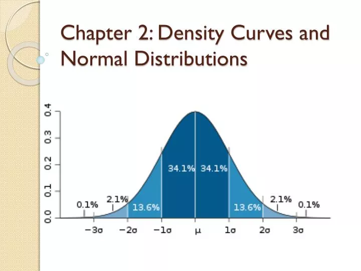
Normal Distributions • 68 – 95 – 99.7 Rule Approximately 68% of the data falls within one standard deviation to the left and right of the mean. Approximately 95% of the data falls within two standard deviations to the left and right of the mean. Approximately 99.7% of the data falls within three standard deviations to the left and right of the mean,
Normal Distributions • The larger the standard deviation is the flatter the bell-shaped curve will be. • The smaller the standard deviation the tighter the data will be. • Inflection points - the first standard deviation to the left and right occur at the inflection points of the graph; the place where the graph switches from concave up to concave down.
Standard Normal Distributions We can standardize data set, so that each data point is represented by number of standard deviations from the mean.
Standard Normal Calculations • If x is an observation from a distribution that has mean μ and standard deviation σ, the standardized value of x is • z = x – μ • σ
Standardizing Data • The heights of young women are approximately normal with μ = 64.5 inches and σ = 2.5 inches. • The standardized height is • z = height – 64.5 • 2.5 • A woman 68 inches tall would have a • z-score of z = 68 – 64.5 = 1.4 • 2.5 • A woman 60 inches tall would have a • Z score of z = 60 – 64.5 = -1.8 • 2.5
Standard Normal Distributions • The standard normal distribution is the normal distribution N(0,1) with mean 0 and standard deviation 1.
Standard Normal Distributions • The standard normal table: • Provides the probability of falling within a certain region of the standard normal distribution. • The distribution provides the area under the curve from - ∞ to some z – score.
Standard Normal Distributions • Find the area under the curve for the following inequalities: • z < 1.52 • z < -1.78 • z > 2.10 • z > -1.23 • -2.10 < z < 1.27 • -1.33 < z < 3.12
Finding Normal Proportions • Step 1 : State the problem in terms of the observed value x. Draw a picture of the distribution and shade the area of interest under the curve. • Step 2 : Standardize x to restate the problem in in terms of standard normal variable z. Draw a picture to show the area of interest under the standard normal curve.
Finding Normal Proportions • Step 3 : Find the required area under the standard normal curve, using Table and the fact that the total area under the curve is 1. • Step 4 : Write your conclusion in the context of the problem.
Example 2.8 The level of cholesterol in the blood is important because high cholesterol levels may increase the risk of heart disease. The distribution of blood cholesterol levels in a large population of people of the same age and sex is roughly normal. For 14 year old boys the mean is μ=170 mg of cholesterol per dl of blood (mg/dl)and the standard deviation is σ=30 mg/dl. Levels above the 240 mg/dl may require medical attention. What percent of 14 year old boys have more than 240 mg/dl of cholesterol?
Example 2.8 • Step 1 : State the problem • P(x>240) with μ=170 mg/dl and σ=30 mg/dl. • Sketch the distribution: mark points of interest and shade the appropriate area. • Step 2 : Standardize x and draw a picture. • Use z conversion formula • Sketch standard normal curve of distribution
Example 2.8 • Step 3 : Use Table appropriately. • 1 – P(z<2.33) • Step 4 : Write your conclusion in context of the problem.
Example 2.9 • What percent of 14 year old boys have blood cholesterol between 170 and 240 mg/dl?
Example 2.9 • Step 1 : State the problem • P(170 < x< 240 • Sketch the curve • Step 2 : Standardize the data • Use z conversion formula • P(0 < z < 2.33) • Sketch the standardized curve • Step 3 : Use the table appropriately • Area between 0 and 2.33 = area below 2.33 – area below 0 • Step 4: State your conclusion in the context of the problem.
Example 2.10 SAT Verbal Scores: Working Backwards • Scores on the recent SAT Verbal test in the recent years follow approximately the N(505,110) distribution. How high must a student score in order to place in the top 10% of all students taking the SAT?
Example 2.10 SAT Verbal Scores • Step 1: State the problem and draw a sketch. • We want a curve that is only .10 of the total area to the right of a z value. • Draw Sketch • z > something, now remember the Table does less than’s only. Step 2: Use the Table. Look in Table A for the entry closest to .9 since that would be the area to the left of our .1 region. z = 1.28 is our standardized score.
Example 2.10 SAT Verbal Scores • Step 3: Unstandardize to transform the z score to a raw data score, x score. • Take our formula z = x – μand solve for x. • σ • x = zσ + μ • x = 1.28 (110) + 505 = 645.8 • Step 4: State the solution in the context of the problem. • A student should score greater than or equal to a 646 to be considered a student in the top 10% of all students taking the SAT Verbal Test.
Assessing Normality • How can we decide if a distribution is normal or not? • Method 1 : Construct a frequency histogram or stem and leaf plot. See if the graph is approximately symmetrical and bell-shaped about the mean. • Histograms can reveal nonnormal features such as outliers, pronounced skewness, or gaps and clusters. • Compare the distribution to the 68 – 95 – 99.7 rule. • Small data sets will rarely be approximately normal due to chance variation.
Assessing Normality • Method 2: Construct a normal probability plot. Put data in from 2.27 page 108 • Put data in List 1 • Use 1 VarStats to compare mean and median. • Construct a dot plot using the 6th option in your StatPlots • Plot the data and zoom in with ZoomStats • If the data is approximately linear then the data is approximately normal.
Calculator Commands Review • normalcdf(xmin, xmax, μ,σ) • normalcdf(zmin,zmax) • shadenorm(xmin,xmax,μ,σ) • Shadenorm(zmin,zmax) • invnorm(p,μ,σ) gives x value that gives this area under the curve • invnorm(p) gives z value with area under the curve.