Download
1 / 29
290 likes | 297 Views
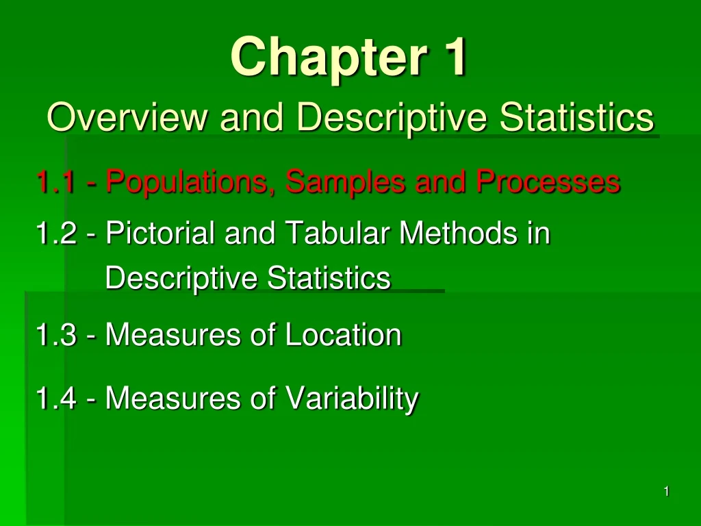
Chapter 1 Overview and Descriptive Statistics. 1.1 - Populations, Samples and Processes 1.2 - Pictorial and Tabular Methods in Descriptive Statistics 1.3 - Measures of Location 1.4 - Measures of Variability.

E N D
Chapter 1Overview and Descriptive Statistics 1.1 - Populations, Samples and Processes 1.2 - Pictorial and Tabular Methods in Descriptive Statistics 1.3 - Measures of Location 1.4 - Measures of Variability
Example: Sample exam scores, n = 20 (“sample size”){60, 60, 70, 70, 70, 70, 70, 70, 70, 70, 80, 80, 80, 80, 90, 90, 90, 90, 90, 90} Because there are many duplicate values, we may construct a table of (absolute) frequencies and corresponding dotplot… R code: x = c(60, 70, 80, 90) freq = c(2, 8, 4, 6) sample = rep(x, freq) stripchart(sample, method = "stack", pch = 19, offset = 1, ylim = range(1, 8))
Example: Sample exam scores, n = 20 (“sample size”){60, 60, 70, 70, 70, 70, 70, 70, 70, 70, 80, 80, 80, 80, 90, 90, 90, 90, 90, 90} Because there are many duplicate values, we may construct a table of (absolute) frequencies and corresponding dotplot… Often though, it is preferable to work with proportions, i.e., relative frequencies… Divide frequencies by n = 20: “Density” All are +, and sum = 1
“Density” = Rel freq / width In general…
“Density” In general…
Example: Sample exam scores, n = 20 (“sample size”){60, 60, 70, 70, 70, 70, 70, 70, 70, 70, 80, 80, 80, 80, 90, 90, 90, 90, 90, 90} 0.40 0.30 0.20 x = c(60, 70, 80, 90) f = c(2, 8, 4, 6) sample = rep(x, f) hist(sample, freq = F, breaks = c(50, 55, 65, 75, 85, 95, 100), labels = T, col = "lightblue") 0.10 Total Area = 1!
{10, 15, 15, 18, 20, 21, 21, 23, 24, 26, 26, 27, 31, 35, 35, 37, 38, 42, 46, 59} {10, 15, 15, 18, 20, 21, 21, 23, 24, 26, 26, 27, 31, 35, 35, 37, 38,42, 46,59} 4 values8 values5 values2 values 1 value From these values, we can construct a table which consists of the frequencies of each age-interval in the dataset, i.e., a frequency table. Frequency Histogram Example: Suppose the random variable isX = Age (years) in a certain population of individuals, and we select the following random sample of n = 20 ages. 8 “Endpoint convention” Here, the left endpoint is included, but not the right. Note!... Stay away from “10-20,” “20-30,” “30-40,” etc. Suggests population may be skewed to the right (i.e., positively skewed). 5 4 In published journal articles, the original data are almost never shown, but displayed in tabular form as above. This summary is called “grouped data.” 2 1
Example: Suppose the random variable isX = Age (years) in a certain population of individuals, and we select the following random sample of n = 20 ages. {10, 15, 15, 18, 20, 21, 21, 23, 24, 26, 26, 27, 31, 35, 35, 37, 38,42, 46,59} As before, it is often preferable to work with proportions, i.e., relative frequencies… Divide frequencies by n = 20. ↓ Relative Frequency Histogram 0.4 0.3 0.2 0.1 0.0 .40 .25 .20 .10 .05 Relative frequencies are always between 0 and 1, and sum to 1.
Example: Suppose the random variable isX = Age (years) in a certain population of individuals, and we select the following random sample of n = 20 ages. {10, 15, 15, 18, 20, 21, 21, 23, 24, 26, 26, 27, 31, 35, 35, 37, 38,42, 46,59} As before, it is often preferable to work with proportions, i.e., relative frequencies… Divide frequencies by n = 20. ↓ “0.00 of the sample is under 10 yrs old” Relative Frequency Histogram 0.4 0.3 0.2 0.1 0.0 “0.20 of the sample is under 20 yrs old” .40 “0.60 of the sample is under 30 yrs old” .25 “0.85 of the sample is under 40 yrs old” .20 “0.95 of the sample is under 50 yrs old” .10 .05 “1.00 of the sample is under 60 yrs old” Relative frequencies are always between 0 and 1, and sum to 1.
Example: Suppose the random variable isX = Age (years) in a certain population of individuals, and we select the following random sample of n = 20 ages. {10, 15, 15, 18, 20, 21, 21, 23, 24, 26, 26, 27, 31, 35, 35, 37, 38,42, 46,59} As before, it is often preferable to work with proportions, i.e., relative frequencies… Divide frequencies by n = 20. ↓ Relative Frequency Histogram 0.4 0.3 0.2 0.1 0.0 .40 .25 .20 .10 (Not a histogram!) .05 “staircase graph” from 0 to 1 Relative frequencies are always between 0 and 1, and sum to 1. Cumulative relative frequencies always increase from 0 to 1.
Example: Suppose the random variable isX = Age (years) in a certain population of individuals, and we select the following random sample of n = 20 ages. {10, 15, 15, 18, 20, 21, 21, 23, 24, 26, 26, 27, 31, 35, 35, 37, 38,42, 46,59} As before, it is often preferable to work with proportions, i.e., relative frequencies… Divide frequencies by n = 20. ↓ Relative Frequency Histogram 0.4 0.3 0.2 0.1 0.0 .40 .25 “staircase graph” from 0 to 1 .20 .10 (Not a histogram!) .05 Relative frequencies are always between 0 and 1, and sum to 1. Cumulative relative frequencies always increase from 0 to 1. But alas, there is a major problem….
Suppose that, for the purpose of the study, we are not primarily concerned with those 30 or older, and wish to “lump” them into a single class interval. {10, 15, 15, 18, 20, 21, 21, 23, 24, 26, 26, 27, 31, 35, 35, 37, 38,42, 46,59} As before, it is often preferable to work with proportions, i.e., relative frequencies… Divide frequencies by n = 20. ↓ What effect will this have on the histogram? Relative Frequency Histogram .40 0.4 0.3 0.2 0.1 0.0 .40 .25 .20 .10 .05 The skew no longer appears. The histogram is distorted because of the presence of an outlier (59) in the data, creating the need for unequal class widths.
(A Pain in the Tuches) Outliers What are they? Informally, an outlier is a sample data value that is either “much” smaller or larger than the other values. How do they arise? experimental error measurement error recording error not an error; genuine What can we do about them? double-check them if possible delete them? include them… somehow perform analysis both ways
Density Histogram 0.04 0.02 0.40 0.0133… 0.20 0.40 IDEA: Instead of having height of each class rectangle = relative frequency, make... areaof each class rectangle = relative frequency. height × = “Density” width = relative frequency / Total Area = 1! width = 10 width = 10 width = 30 The outlier is included, and the overall skewed appearance is restored. Exercise: What if the outlier were 99 instead of 59?
Density Histogram 0.04 0.04 0.02 0.40 Question: Approx what proportion of the sample is between 18-24 yrs old (inclusive)? 0.0133… 0.20 0.02 0.40 0.40 Step 1. Identify the intervals & rectangles. Step 2. Split the FIRST rectangle at 18 as shown. • Step 3. Observe that… • the interval [18, 20) has width = 2 years • the interval [10, 20) has width = 10 years. • The ratio = 2/10 = 1/5. 0.20 Step 4. Therefore, the redarea = 1/5 of .20 = .04. Step 5. Repeat Steps 2-4 for SECOND rectangle at 24. The redarea = 2/5 of .40 = .16. Step 6. ADD: .04 + .16 = .20 i.e., 20%
Density Histogram 0.04 0.04 0.02 0.40 Question: Approx what proportion of the sample is between 18-24 yrs old (inclusive)? 0.0133… 0.20 0.02 0.40 0.40 Step 1. Identify the intervals & rectangles. - OR - Step 2. Use “Density = Area / Width” (see page 2.3-5 of the posted Lecture Notes): 0.20 FIRST area = Width Density = (20 – 18)(.02) = .04 SECOND area = Width Density = (24 – 20)(.04) = .16 Exercise: Confirm that the actual proportion = 30%. Step 3. ADD: .04 + .16 = .20 i.e., 20% Exercise: What if ages 23, 24 were both changed to 25?
Chapter 1Overview and Descriptive Statistics 1.1 - Populations, Samples and Processes 1.2 - Pictorial and Tabular Methods in Descriptive Statistics 1.3 - Measures of Location 1.4 - Measures of Variability
Center “Measures of ” Example: Sample exam scores {60, 60, 70, 70, 70, 70, 70, 70, 70, 70, 80, 80, 80, 80, 90, 90, 90, 90, 90, 90} • sample mode most frequent value = 70 • sample median “middle” value = (70 + 80)/2 = 75 • sample mean average value = Useful when outliers are present, e.g., employee salaries + CEO Quartilesare found similarly: Q1 = 70, Q2 = 75, Q3 = 90 Quintiles, deciles, other percentiles (= quantiles) similar. 1/20 (60)(2) + (70)(8) + (80)(4) + (90)(6) = 77 xifi x =
“Measures of Center” Example: Sample exam scores {60, 60, 70, 70, 70, 70, 70, 70, 70, 70, 80, 80, 80, 80, 90, 90, 90, 90, 90, 90} • sample mode most frequent value = 70 • sample median “middle” value = (70 + 80)/2 = 75 • sample mean average value = 1/20 (60)(2) + (70)(8) + (80)(4) + (90)(6) = 77 xifi x =
“Measures of Center” Example: Sample exam scores {60, 60, 70, 70, 70, 70, 70, 70, 70, 70, 80, 80, 80, 80, 90, 90, 90, 90, 90, 90} • sample mean 1/20 (60)(2) + (70)(8) + (80)(4) + (90)(6) = 77 2 20 8 20 4 20 6 20 1/20 (60)(2) + (70)(8) + (80)(4) + (90)(6) xip(xi) xifi “weighted” sample mean (with weights = relfreqs) x = x = “Notation, notation, notation.”
“Measures of ” Spread Example: Sample exam scores {60, 60, 70, 70, 70, 70, 70, 70, 70, 70, 80, 80, 80, 80, 90, 90, 90, 90, 90, 90} … but how do we measure the “spread” of a set of values? • sample mean • First attempt: • sample range=xn – x1= 90 – 60 = 30. Simple, but… Ignores all of the data except the extreme points, thus far too sensitive to outliers to be of any practical value. Example: Company employee salaries, including CEO • Can modify with… • sample interquartile range (IQR) = Q3 – Q1 • = 90 – 70 = 20. We would still prefer a measure that uses all of the data.
“Measures of Spread” Example: Sample exam scores {60, 60, 70, 70, 70, 70, 70, 70, 70, 70, 80, 80, 80, 80, 90, 90, 90, 90, 90, 90} … but how do we measure the “spread” of a set of values? • sample mean Better attempt: Calculate the average of the “deviations from the mean.” 1/20 [(–17)(2) + (–7)(8) + (3)(4) + (13)(6)] = 0. ???????? This is not a coincidence – the deviations always sum to 0* – so it is not a good measure of variability. (xi– x) fi = 0.40 * The sample mean is a “balance point” for the data. Question: Why wouldn’t the median 75 be the balance point? 0.30 0.20 0.10 See Prob2.5 / 11 in Lec Notes for a more obvious example.
“Measures of Spread” Example: Sample exam scores {60, 60, 70, 70, 70, 70, 70, 70, 70, 70, 80, 80, 80, 80, 90, 90, 90, 90, 90, 90} “typical” sample value • sample mean a modified average of the “squared deviations from the mean.” Calculate the [(–17)2(2) + (–7)2(8) + (3)2(4) + (13)2(6)] 1/19 = 106.316 • sample variance (xi– x)2fi s2 = • sample standard deviation s = s = 10.311 “typical” distance from mean
Grouped Data - revisited Use the interval midpoints for
Grouped Data - revisited 15 25 45 Use the interval midpoints for Compare this “grouped mean” with the actual sample mean.
Grouped Data - revisited Use the interval midpoints for 0.04 Compare this “grouped mean” with the actual sample mean. median Q2 = ? 0.3 0.1 Step 1. Identify the interval & rectangle. 0.02 Step 2. Split the rectangle so that 0.5 area lies above and below. 0.40 0.0133… 0.20 0.40
Grouped Data - revisited 0.3 0.1 0.1 0.1 0.1 Use the interval midpoints for Compare this “grouped mean” with the actual sample mean. median Q2 = ? Step 1. Identify the interval & rectangle. Step 2. Split the rectangle so that 0.5 area lies above and below. …OR… Step 3. Observe that this rectangle can be split into 4 strips of 0.1 each. 22.5 25 27.5 Step 4. Thus, split the interval into 4 equal parts, each of width (30 – 20 )/4 = 2.5 years. 00 00
Grouped Data - revisited 0.3 0.1 Use the interval midpoints for • Other percentiles are done similarly. • Solve using cumul dist, w/o histogram …see posted Lecture Notes! Compare this “grouped mean” with the actual sample mean. median Q2 = ? Step 1. Identify the interval & rectangle. Step 2. Split the rectangle so that 0.5 area lies above and below. …OR… Step 3. Set up a proportion and solve for Q: …OR… 00 00 Label as shown, and use the formula .
Comments • is an unbiased estimator of the population mean , s2 is an unbiased estimator of the population variance 2. (Their “expected values” are and 2, respectively.) • Beware of roundoff error!!! There is an alternate, more computationally stable formula for sample variance s2. • The numerator of s2 is called a sum of squares(SS); the denominator “n – 1” is the number of degrees of freedom(df) of the n deviations xi – , because they must satisfy a constraint (sum = 0), hence 1 degree of freedom is “lost.” • A natural setting for these formulas and concepts is geometric, specifically, the Pythagorean Theorem: a 2 + b 2 = c 2. See lecture notes appendix… c b a