Download

1 / 11
110 likes | 221 Views
Class Notes on Nonlinear Regression (Chapter 5). Reminders: Homework 3 on Design due on Friday 22nd February. First Exam is on Thursday 28th February. Homework 4 on GdLM’s due on Friday 14th March. Thursday 21st February Class

E N D
Class Notes on Nonlinear Regression (Chapter 5) • Reminders: • Homework 3 on Design due on Friday 22nd February • First Exam is on Thursday 28th February • Homework 4 on GdLM’s due on Friday 14th March
Thursday 21st February Class • Nonlinear models often result from compartmental models (scientific “common sense”), and the parameters are usually very important and interpretable (as compared with linear models) • Need to give starting values, and that requires understanding the model function and sometimes some ingenuity (p.4) • Iterate to a solution using e.g. MGN method – results in parameter estimation, and then interpretation or prediction • Rival model functions exist for the same dataset – e.g., SE2, MM2 (Michaelis-Menton), and Lansky model functions all look very similar (like the figure at the bottom of p.7)
Thursday 21st February Class • CI’s: two types – Wald (estimate +/- t*SE) is based on a parabolic approximation to the SSE or likelihood, and Likelihood-based. PLCI’s are often asymmetric, which makes more sense since usually our information about a parameter is asymmetric. Best to use PLCI’s, but they are a pain to find. The difference between WCI’s (Wald) and PLCI’s depends upon “curvature” – more on this later. • Better understanding of MM2 model function parms, and how to give good starting values
Example 5.2 – linear model, but nonlinear model is appropriate since we are interested in the intraclass correlation (p.13), which is a nonlinear function of the linear model parameters. Find the PLCI from the graph on p.12 bottom; = 0.811 occurs where this plot hits its maximum • Thursday 21st February Class • Example 5.1 BOD – pp. 7-11: parameter estimation, WCR for q, LBCR for q, PLCI’s for individual parameters (graph p.10 bottom), WCI’s for individual parameters from a parabolic approximation – recapped in Tables on p.12
Thursday 21st February Class • Example 5.3 (Laetisaric acid) another linear model ‘reparameterized’ into a nonlinear one; here again, Wald and Likelihood intervals really do differ – use PLCI’s when available • Example 5.4 – two treatment groups (conv vs. eshb) fitting a 3-parameter curve to each and testing for common parameters. Compound hypothesis (bottom of p.17) is tested using the Full-and-Reduced F statistic, F2,18 = [(0.2465-0.1737)/2] / [0.1737/18] = 3.772, which carries a p-value of 0.0428.
Tuesday 26th February Class • Ex. 5.5 – downward SE2 doesn’t fit (see residuals on p.20), but SE2 with a lag (“variable knot”) does fit: 95% WCI for knot extends from 25.16 minutes to 46.19 minutes • Ex. 5.6 – another lag example • Ex. 5.7 – Fitting a (modified) LL4 model function for May and one for June; wish to test H0: q1M = q1J, q2M = q2J andq3M = q1J; tested using Full-and-Reduced F statistic, F3,24 = [(0.0206-0.0179)/3] / [0.0179/24] = 1.20, which carries a p-value of 0.329. We retain the claim of common upper and lower asymptotes and slopes for M and J.
Tuesday 26th February Class • All our models so far are homoskedastic normal NLINs, but data in Ex. 5.8 show non-constant variance. Letting “rhs” denote the (mean) model function, we propose that VAR = s2*rhsr, where r is an additional parameter to be estimated. The case where r = 0 is then constant variances across X. To test H0: r = 0, we use Wald or LR. Wald gives t55 = 1.4707/0.4699 = 3.13 and p = 0.0028. More reliable is the LR test c2 = 254.0 – 245.3 = 8.7 and p = 0.0032. (That Wald gives a similar p-value means quadratic approx. is good here.) Regardless, we reject the null, and accept heteroskedasticity. One of the ramifications is that the SE for the LD50 drops from 0.3805 to 0.3297 (drops 13.4%).
Tuesday 11th March Class • Today, exponential family (but non-Gaussian) NLModels • Example 5.10 - return to Menarche example but with LD50 = g as a new model parameter; now, SAS gives a 95% WCI for g in the NLMIXED output. We could also find a PLCI • Return to Budworms example in Example 5.11 – we accept common slopes using the –2DLL c2 test (p = 0.1797 on p.30) • Grauer Logistic curve doesn’t fit (see residuals on p.31) when using x = age at death. Output 5.10c indicates that we should use the log-age scale, and new model is Equation (5.25). Then, LD50 is estimated as 10.9717 years.