Download
1 / 38
380 likes | 383 Views
Atmospheric Aerosol Attenuation Measurements at the Pierre Auger Observatory. Laura Valore University of Naples & INFN Naples. AtmoHEAD workshop – CEA Saclay - June 10 2013. Outlook. The Pierre Auger Observatory

E N D
Atmospheric Aerosol Attenuation Measurements at the Pierre Auger Observatory Laura Valore University of Naples & INFN Naples AtmoHEAD workshop – CEA Saclay - June 10 2013
Outlook • The Pierre Auger Observatory • The effect of aerosol attenuation on air fluorescence measurements • The Central Laser Facilities (CLF) and the eXtreme Laser Facility (XLF) of the Pierre Auger Observatory • Hardware • Operation • 9 years of results : 2004-2012 aerosol attenuation profiles • analyses techniques • determination of uncertainties • comparison of results • the Pierre Auger Observatory Aerosol Database
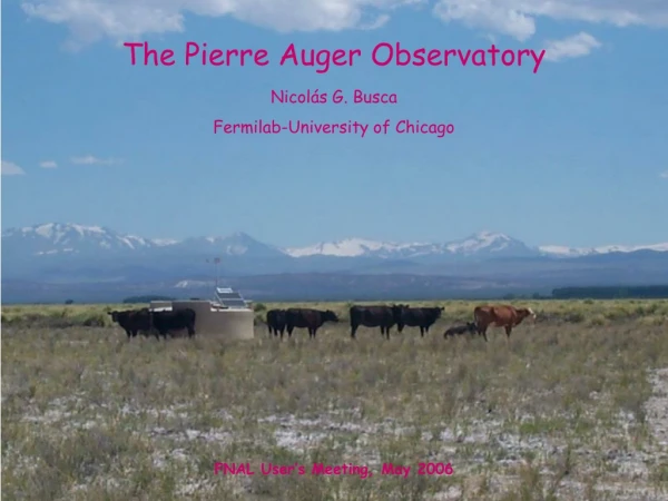
The Pierre Auger Observatory Malargue, Argentina 1660 water Cerenkov detectors distributed over an area of 3000 km2 + 24+3 UV telescopes, positioned at 4+1 sites around the edge of the ground array Installation completed in november 2008
The Hybrid Detector Two independent and complementary detection techniques Surface Detector (SD) (density of particles at ground) Fluorescence Detector (FD) (longitudinal development of showers) A nearly calorimetric measurement of the energy is performed, since the flux of fluorescence photons produced during the development of the shower is proportional to dE/dX, the energy deposit per unit slant depth of the traversed atmosphere the calorimeter (the atmosphere) properties needs to be well known !
Iλ(s) = I0λ (s) Tλmol(s) Tλabs(s) Tλaer (s)(1+f)(dΩ/4π) The calorimeter properties the atmosphere is responsible for production and attenuation of UV light. • production : the yields of light from Cerenkov and fluorescence emission processes depend on molecules in atmosphere • attenuation : the attenuation of light in the atmosphere depend mainly on molecules and aerosols. It can be factorized into separate molecular and aerosol components Tmol and Taer (+Tabs) : • Tmolcan be analitically measured from ballons measurements or satellite data • Tabs > 0.999 for λ > 340 nm (Ozone) below 15 km (therefore neglected) • Taer determination depends on frequent field measurement of the vertical aerosol optical depth VAOD(h, λ), due to the rapidly changing conditions (time scale of 1 hour or less) Tλaer(s) = exp (-VAOD(h, λ)/senθ)
The effect of aerosol conditions on air fluorescence measurements • 20% of showers need a >20% energy correction • 7% of showers need a >30% energy correction • 3% of showers need a >40% energy correction Neglecting the presence of aerosols causes an underestimate in energy on average from 8% (at lower energies) to 25% (at higher energies) Neglecting the presence of aerosols causesa systematic shift in Xmax from -1 g/cm2 at lower energies to 10 g/cm2 at higher energies from The Pierre Auger Collaboration, Astroparticle Physics 33 (2010) 108-129
The Aerosol Monitoring System The Pierre Auger Observatory operates an array of monitoring devices to record the atmospheric conditions. Most of instruments are used to estimate the hourly aerosol transmission between the point of production of the fluorescence light and the FD: as explained, if not properly taken into account, these dynamic conditions can bias showers reconstruction. Central Laser Facility LIDAR IR cloud camera
Instruments to measure the aerosol attenuation TheCentral Laser Facility (CLF)and theeXtreme Laser Facility (XLF)produce laser beams from a position nearly in the center of the array. Once the nominal energy of the laser source is known, the amount of photons reaching the FDs depends on the atmospheric conditions, and theaerosol transmissioncan be inferred; alsocloudscan be detected. Four LIDAR stations, one for each FD site, are equipped with a UV laser source for the detection of the elastic backscattered light to record local aerosol conditions and clouds. They can also provide rapid monitoring mode after the detection of high-energy showers. A Raman LIDAR station is also present at one of the four FD sites. The on-going upgrade of the CLF includes the addition of a Raman LIDAR at the CLF site. 4
Instruments to measure the aerosol attenuation The Central Laser Facility (CLF) and the eXtreme Laser Facility (XLF) produce laser beams from a position nearly in the center of the array. Once the nominal energy of the laser source is known, the amount of photons reaching the FDs depends on the atmospheric conditions, and the aerosol transmission can be inferred; also clouds can be detected. Four LIDAR stations, one for each FD site, are equipped with a UV laser source for the detection of the elastic backscattered light to record local aerosol conditions and clouds. They can also provide rapid monitoring mode after the detection of high-energy showers. A Raman LIDAR station is also present at one of the four FD sites. The on-going upgrade of the CLF includes the addition of a Raman LIDAR at the CLF site. 4
Instruments to measure the aerosol attenuation The Central Laser Facility (CLF) and the eXtreme Laser Facility (XLF) produce laser beams from a position nearly in the center of the array. Once the nominal energy of the laser source is known, the amount of photons reaching the FDs depends on the atmospheric conditions, and the aerosol transmission can be inferred; also clouds can be detected. Four LIDAR stations, one for each FD site, are equipped with a UV laser source for the detection of the elastic backscattered light to record local aerosol conditions and clouds. They can also provide rapid monitoring mode after the detection of high-energy showers. A Raman LIDAR station is also present at one of the four FD sites. The on-going upgrade of the CLF includes the addition of a Raman LIDAR at the CLF site. 4
The Central Laser Facility (CLF) and the eXtreme Laser Facility (XLF) • Nd::YAG laser source @ 355nm • Distance from FD buildings between 26km and 40km • Position, direction and energy known CLF
CLF hardware The CLF system is described in : JINST 1 P11003 (2006)“The Central Laser Facility at the Pierre Auger Observatory” The trajectory of the vertical beam is shown. The dashed line indicates the fraction of the laser beam going into the pyroelectric probe for the relative shot by shot calibration.
CLF calibration system Relative and absolute energy calibration of the laser are mandatory! The sky energy of each shot must be known with the highest precision for aerosol profiles measurements. I The laser energy of the CLF is monitored by two pick-off probes inside the optical table : a photodiode ad a pyroelectric probe. The second one is used for the relative calibration since 2005. In addition, absolute calibrations were periodically performed. BUT ! In these 9 years (from 2004), dust accumulating on the last mirror of the optical table, downstream the probe, caused a reduction of the effective energy sent to the sky that was revealed by absolute calibration measurements. Since 2010, monthly absolute calibrations are performed at the CLF to trace this trend accurately
XLF calibration system Relative calibration : pyroelectric probe Absolute calibration : a robotic arm moves a calibration probe in the beam path of the laser at least twice per night !
Laser Facilities and the FD • CLF/XLF operation (during FD acquisition): • Completely automated operation • 50 vertical shots every 15 minutes, a shot every 2 seconds, average energy 6.5 mJ • 2 sets of 1 hour inclined shots Photons@FD vs time
Laser vs Shower Events The amount of light scattered out of a 6.5 mJ UV laser beam is almost equivalent to the amout of fluorescence light produced by a 5x10¹⁹ eV shower at a distance of 16km from the telescope
laser-based methods for the determination of the atmospheric aerosol attenuation Laser light is attenuated in the same way as fluorescence light as it propagates towards the FD. Measuring the amount of photons reaching the FD allows one to evaluate the attenuation in atmosphere due to aerosols JINST 8 P04009 (2013) Data Normalized Analysis the aerosol attenuation is measured by comparing laser events with those of a reference purely molecular night in which the aerosol attenuation is negligible (Rayleigh Night) Laser Simulation Analysis the aerosol attenuation is measured by comparing measured and simulated laser events in different atmospheric conditions, described by a two parameters model.
Laser Simulation & Data Normalized Analyseswhat they have in common To minimize fluctuations, both analyses make use of average profiles of light measured at the aperture of the FD buildings, normalized to a reference energy Measures profiles are affected by unavoidable systematics related to FD and laser calibrations; simulated profiles are affected by systematics related to the simulation procedure; using measurements recorded on extremely clear nights where molecular Rayleigh scattering dominates, laser observations can be normalized without the need for absolute photometric calibrations of the FD or laser.
Rayleigh Night identification These “reference clear nights” are identified using a procedure looking for profiles with • maximum photon transmission • maximum compatibility with the shape of a profile simulated in conditions with negligible aerosol attenuation (Kolmogorov-Smirnov test) The procedure is repeated for each FD telescope, for both laser facilities. One reference clear night per year is identified. Cross-checks with data from the Aerosol Phase Function monitor are performed to confirm the validity of the chosen Rayleigh Nights.
Data Normalized Analysisbuilding hourly profiles and marking clouds The procedure starts building quater-hour profiles of light collected at the aperture of the FD building corresponding to the 50 laser shots. Profiles are normalized to 1mJ. Clouds are then marked by comparing the photon transmission of the quarter-hour profiles to that of the clear profile. The ratio Tquarter/Tclean is used to identify clouds and set the minimum cloud layer altitude. Hours are marked as cloudy only if clouds are found in at least two quarter-hour sets. After cloud identification, the full hour profile is built averaging all quarter-hour profiles available.
Data Normalized Analysismeasuring the aerosol attenuation profiles aer(h) Using vertical laser shots, and taking into account the laser – FD geometry, the vertical aerosol optical depth is : Where Nmol(h) is the number of photons of the reference clear night, Nobs(h) is the number of photons of the measured hourly profile in analysis and φ2 is the elevation angle A first guess of aer(h) , named measaer(h), is measured for each bin
Data Normalized Analysismeasuring the aerosol attenuation profiles aer(h) To take into account also the aerosol scattering from the laser beam, an iterative procedure is applied to differentiate measaer(h) to obtain the aerosol extinction α(h) for each bin, in which it can be assumed as constant. After a number of iterations, the final α(h) is integrated to obtain the fitaer(h) • Black traces show measaer(h) (with upper and lower bounds) • Red traces represent fitaer(h)
Laser Simulation Analysisthe parametric model of the aerosol attenuation The method is based on the comparison between measured and simulated events. Simulated laser events are generated at a fixed energy using a parametric description of the aerosol attenuation. The vertical aerosol optical depth is described with a function of two parameters: Laer, the aerosol horizontal attenuation length Haer, the aerosol scale height A third parameter, the aerosol mixing layer height, taking into account the Planetary Boundary Layer, will be added to this model.
Laser Simulation Analysisbuilding quarter hour profiles and simulations the relative energy scale between measured and simulated events is set using the normalization to the reference clear night. Quarter-hour profiles are built averaging over 50 shot groups, normalizing each profile to 6.5 mJ. Simulations are generated in groups of fifty events at 6.5 mJ. GRID FEATURES : Lmie : 5km – 50km , step 1.25km Lmie : 50km – 150km, step 2.5km Hmie : 500m - 5km , step 250m A grid is produced for each laser facility, for each FD site and for each month using molecular monthly density profiles.
Laser Simulation Methodmeasuring the aerosol attenuation profiles aer(h) Each measured profile is compared to the whole grid of simulations. The simulated profile that best matches the measured one is chosen minimizing the square difference of the number of photons per each bin. The Laer and Haer parameters of the chosen best simulated profile are used to measure the aerosol attenuation profile Clouds are identified working on the profile of the difference between the measured and best simulated profile. With this choice, the baseline is close to zero and the peaks and holes in the signal are clearly visible. The signal to noise ratio and the highest/lowest signal are used to mark the cloud lowest layer height, and the maximum height of the aerosol profile measured
Data Normalized Analysis Laser Simulation Analysis
Hazy atmo laser profiles Average clean atmo laser profiles
Statistical and systematic uncertainties Various uncertainties were identified in the methods fot the determination of the aer(h), that are listed below. The uncertaintiesare separated into statistical and systematic contributions. Assignments were based on whether the effect of the uncertainty would be correlated over a given shower data sample, or largely uncorrelated from one air shower event to the next.
Correlated / Systematics Relative laser energy (1 - 2.5% CLF, 1% XLF) and FD calibration (2%) : describe how accurately variations in the laser energy and FD calibration were tracked between reference nights, which are one year apart Reference night (3%) : systematics related to the choice of the Rayleigh Night Uncorrelated / Statistical Relative laser energy (2%) : statistical variations of the relative energy probe Relative FD calibration (4%) : it includes an estimate of the variabiliy of the calibration value Atmospheric Fluctuation within hour (3%) : estimated on an event-by-event basis
2004 – 2012 aerosol attenuation profiles • The hourly aerosol attenuation over 9 years have been measured using the two analyses described. The compatibility of the results obtained is shown The spread of the points is within the systematic error bands. More than 6000 hours are shown in this plot.
An example of aerosol attenuation profile in average aerosol attenuation conditions measured with the two analyses described, together with correlated (systematic) and uncorrelated (statistical) errors
9 years of aerosol attenuation profiles measured. A total of 10430 hours have been measured for the Los Leones site, 9302 for Los Morados, 2270 for Loma Amarilla (started in 2010) and 10430 for Coihueco, using results from the DN analysis + filling the gaps with results from the LS analysis
Auger Aerosol Database In the aerosol database the atmosphere is described by 5 vertical sections. At each section, α(z) and aer(h)in steps of Δh = 200 m are associated for each hour The present aerosol database is filled with more than 30000 hours of VAOD profiles and is currently used for EAS analysis. Due to the distance, XLF data are used to produce aerosol attenuation profiles from Loma Amarilla, while CLF data are used for Los Leones, Los Morados and Coihueco
Conclusions • The Pierre Auger Observatory uses hourly aerosol attenuation measurements, obtained analyzing events from the two laser facilities, to perform precise measurements of the energy and Xmax of showers • Two analyses are used to measure the vertical aerosol optical depth profiles. The high compatibility of the two analysis is proved. • 9 years of aerosol profiles are stored in the aerosol database and used for showers analysis : • more than 30000 hours • more than 5 millions of laser shots
The Fluorescence Detector During the development of an EAS particles interact with N2, O2 molecules Excited molecules can dissipate energy emitting photons in the range of ultraviolet or in the visible, determining the production of fluorescence light At E>1017 eV the production of fluorescence light is enough to be detected.
Rayleigh Night identification Mainly based on the analysis of a molecular profile shape • Simulation of an average Rayleigh profile at 6.5 mJ for each monthly density profile • For each month, the simulated Rayleigh profile is compared to all 6.5mJ normalized real profiles • The comparison returns: • thepseudo-probabilitythat the analyzed profile to be compatible to the Rayleigh one (Kolmogorov Test) • theratioof the total number of photons of the measured profile with respect to that of the “Rayleigh” profile The ratio returns the normalization constant that fixes the energy scale needed in the Laser Simulation analysis.
Rayleigh Night identification (2) For each calibration epoch the search for the Rayleigh night is performed among profiles having high values of both probability and ratio a “search region” is defined profiles belonging to the search region are grouped by night: nightly average Probability andRatioare computed a list of candidate Rayleigh nights is produced the night with the highest probability and at least 4 quarter-hours measurements is selected as the Rayleigh night Selected Rayleigh nights have been checked with other instruments Rayleigh nights from different eyes have been checked to be consistent