Download
1 / 37
370 likes | 565 Views
Lecture 8 Logic/Circuit Synthesis for Low-Power. Michael L. Bushnell CAIP Center and WINLAB ECE Dept., Rutgers U., Piscataway, NJ. Logic Level Optimizations Circuit Level Optimizations Summary. Logic-Level Optimizations. Design Flow. Behavioral Synthesis – not used very much

E N D
Lecture 8Logic/Circuit Synthesis for Low-Power Michael L. Bushnell CAIP Center and WINLAB ECE Dept., Rutgers U., Piscataway, NJ • Logic Level Optimizations • Circuit Level Optimizations • Summary Analog and Low-Power Design Lecture 8 (c) 2003
Logic-Level Optimizations Analog and Low-Power Design Lecture 8 (c) 2003
Design Flow • Behavioral Synthesis – not used very much • Initial design description: RTL or Logic level • Logic synthesis widely used • FSMs: • State Assignment – opportunity for power saving • Logic Synthesis – look for common subfunctions – opportunity for power saving • Custom VLSI design – size transistors to optimize for power, area, and delay • Library-based design – technology mapping used to map design into library elements Analog and Low-Power Design Lecture 8 (c) 2003
FSM and Combinational Logic Synthesis • Consider likelihood of state transitions during state assignment • Minimize # signal transitions on present state inputs V • Consider signal activity when selecting best common sub-expression to pull out during multi-level logic synthesis • Factor highest-activity common sub-expression out of all affected expressions Analog and Low-Power Design Lecture 8 (c) 2003
Huffman FSM Representation Analog and Low-Power Design Lecture 8 (c) 2003
Probabilistic State Transition Graphs (STGs) • Edges showing state transitions not only indicate input values causing transitions and resulting outputs • Also have labels pijgiving conditional probability of transition from state Si to Sj • Given that machine is in state Si • Directly related to signal probabilities at primary inputs • Introduce self-loops in STG for don’t care situations to transform incompletely-specified machine into completely-specified machine Analog and Low-Power Design Lecture 8 (c) 2003
Example Analog and Low-Power Design Lecture 8 (c) 2003
Relationship Between State Assignment and Power • Hamming distance between states Siand Sj: • H (Si, Sj) = # bits in which the assignments differ • Average Power: • D (i) = signal activity at node i • Approximate Ci with fanout factor at node i • Average power proportional to: Analog and Low-Power Design Lecture 8 (c) 2003
Handling Present State Inputs • Find state transitions (Si, Sj) of highest probability • Minimize H (Si, Sj) by changing state assignment of Si, Sj • Requires system simulation of circuit over many clock periods, noting signal values and transitions • If one-hot design is used, note that H = 2 for all states • Impossible to obtain optimum power reduction • Uses too many flip-flops • Optimization cost function: Analog and Low-Power Design Lecture 8 (c) 2003
Simulated Annealing Optimization Algorithm • Allowed moves: • Interchange codes of two states • Assign an unassigned code to a state that is randomly picked for an exchange • Accept move if it decreases g • If move increases g, accept with probability: e - |d (g) | / Temp Analog and Low-Power Design Lecture 8 (c) 2003
Example State Machine Analog and Low-Power Design Lecture 8 (c) 2003
State Assignments • Coding 1 uses 15% more power than coding 2 Analog and Low-Power Design Lecture 8 (c) 2003
Multi-Level Logic Optimization for Low Power • Combinational logic is F (I, V) • I = set of primary inputs • V = present state inputs • Need to estimate probabilities and activities of V inputs (same as next state outputs but delayed one clock period) in order to synthesize logic for minimum power • Use methods of Chapter 3 • Randomly generate PI signals with probabilities and activities conforming to a given distribution • Get D (vj) = transition activity at input vj (transitions / clock period) • Get from fast state transition diagram simulation Analog and Low-Power Design Lecture 8 (c) 2003
Power-Driven Multi-Level Logic Optimization • Use Berkeley MIS tool • Takes set of Boolean functions as input • Procedure kernel finds all cube-free multiple or single-cube divisors of each Boolean function • Retains all common divisors • Factors out best few common divisors • Substitution procedure simplifies original functions to use factored-out divisor • Original criteria for selecting common divisor: • Chip area saving • New criterion: power saving Analog and Low-Power Design Lecture 8 (c) 2003
Boolean Expression Factoring • g = g (u1, u2, …, uK), K 1 is common sub-expression • When g factored out of L functions, signal probabilities and activities at all circuit nodes are unchanged • Capacitances at output of driver gates u1, u2, …, uK change • Each drives L-1 fewer gates than before • Reduced power: • D (x) = activity at node x • nui = # gates belonging to node g and driven by uK Analog and Low-Power Design Lecture 8 (c) 2003
Factoring (continued) • Only one copy now of g instead of L copies • L-1 fewer copies of internal nodes v1, v2, …, vm in factored-out hardware for switching and dissipating power • Power saving: • Total power saving: Analog and Low-Power Design Lecture 8 (c) 2003
Factoring (concluded) • T (g) = # literals in factored form of g • Area saving: • Net saving of power and area: Analog and Low-Power Design Lecture 8 (c) 2003
Optimization Algorithm Analog and Low-Power Design Lecture 8 (c) 2003
Optimization Algorithm (concluded) Analog and Low-Power Design Lecture 8 (c) 2003
Example Unoptimized Circuit Analog and Low-Power Design Lecture 8 (c) 2003
Optimization for Area Alone Analog and Low-Power Design Lecture 8 (c) 2003
Optimization for Low-Power Alone • Large area but reduces power from 476.12 to 423.12 Analog and Low-Power Design Lecture 8 (c) 2003
Results • On the MCNC Benchmarks: • Two-stage process • State assignment problem • Multi-level combinational logic synthesis based on power dissipation and area reduction • Result: • 25% reduction in power • 5% increase in area Analog and Low-Power Design Lecture 8 (c) 2003
Technology Mapping for Low Power • Problem statement: • Given Boolean network optimized in a technology-independent way and a target library, bind network nodes to library gates to optimize a given cost • Method: • Decompose circuit into trees • Use dynamic programming to cover trees • Cost function: • Traverse tree once from leaves to root Analog and Low-Power Design Lecture 8 (c) 2003
Extension for Low-Power Design • Power dissipation estimate: • Estimate partial power consumption of intermediate solutions • Cost function: • MinPower (ni) is minimum power cost for input pin ni of g • power (g) = 0.5 f VDD2 ai Ci • Formulation: • R = Total Area, w gives their relative importance Analog and Low-Power Design Lecture 8 (c) 2003
Top-Level Mapping Algorithm • Overall process: • From tree leaves to root, compute trade-off curves for matching gates from library • From root to leaves: • Select minimum-cost solution • Reduces average power by 22% while keeping the same delay • Sometimes increases area as much as 39% Analog and Low-Power Design Lecture 8 (c) 2003
Circuit-Level Optimizations Analog and Low-Power Design Lecture 8 (c) 2003
Algorithm Components • Find which gate to examine next • Use a set of transformations for the gate • Compute overall power improvement due to transformations • Update the circuit after each transformation Analog and Low-Power Design Lecture 8 (c) 2003
Gate Delay Model • For every input terminal Ii and output terminal Ojof every gate: • T ii,j (G) – fanout load independent delay (intrinsic) • Ri,j (G) – additional delay per unit fanout load • Total gate propagation delay from input to output: • Normalize all activities dy by dividing them by clock activity (2f) • Probability of rising or falling transition at y: Analog and Low-Power Design Lecture 8 (c) 2003
CMOS Gate Usage • Deep sub-micron technology: • Delay of NAND/NOR to INVERTER delay lessens in deep sub-micron technology • Series transistor connection Vds and Vgs smaller than that for inverter transistor • Encourages wider use of complex CMOS gates • Important to order series transistors correctly • Delay varies by 20% • Power varies by 10% Analog and Low-Power Design Lecture 8 (c) 2003
CMOS Gate Power Consumption • For series-connected transistors, signal with lower activity should be on transistor closest to power supply rail Analog and Low-Power Design Lecture 8 (c) 2003
Calculating Transition Probability • Hard to find pzi • Hard to determine prior state of internal circuit nodes • Assume that when state cannot be determined, a transition occurred (upper power limit) • More accurate bound: Observe that # conducting paths from node to Vdd must change from 0 to > 0 followed by similar change in # conducting paths to Vss • Use # conducting paths that is smaller • Use serial-parallel graph edge reduction techniques Analog and Low-Power Design Lecture 8 (c) 2003
Transistor Reordering • Already know delay of longest paths through each gate input from static timing analyzer • Should (for NAND or NOR) connect latest arriving signal to input with smallest delay • Break gate inputs into permutable sets and swap inputs • Hard to compute which input order is best – can afford to enumerate all possible orderings and try them • Compute prob. (signal is switching while all other signals in permutable set are on) – gives maximum internal node C charging / discharging Analog and Low-Power Design Lecture 8 (c) 2003
Optimization Algorithm • Try to meet circuit performance goal (do forwards and then backwards graph traversal) • During backwards traversal: • If a gate delay is larger than specified delay, reorder inputs to decrease delay • End up with valid backwards delays for gates, but not valid forward delays • Repeat forward traversal if input reordering was done • Continue reordering inputs if gate path delay specification is exceeded • Continue alternating forward/backwards traversals until no more reorderings happen, then proceed to power minimization Analog and Low-Power Design Lecture 8 (c) 2003
Power Minimization • Repeat alternating forward and backward traversals • Change: Determine delay increase for input order corresponding to least estimated power dissipation • If increase less than available path slack, reorder inputs • Available slack: difference between: • Larger of maximum acceptable delay and longest path delay • Delay of longest path through gate • Results on MCNC benchmarks – reduced power by 7 to 8 %, with no critical path delay increase, and very little area penalty Analog and Low-Power Design Lecture 8 (c) 2003
Transistor Resizing Methods • Datta, Nag & Roy: resized transistors on critical paths to reduce power and shorten delay • Wider transistors speed up critical path and reduce power because you get sharper edges, and therefore less short-circuit power dissipation • Penalty – larger transistors increase node C, which can increase delay and power • Increased drive for present block, and greater transition time for preceding block (due to larger load CL) may increase present block short-circuit current • Simulated annealing algorithm tries to optimize gates on N most critical paths Analog and Low-Power Design Lecture 8 (c) 2003
Summary • Logic-level multi-level logic optimization is effective • State assignment • Modified MIS algorithm • Logic-level Technology mapping • Tree-covering algorithm is effective • Circuit-level operations are effective • Transistor input reordering • Transistor resizing Analog and Low-Power Design Lecture 8 (c) 2003