Download
1 / 7

E N D
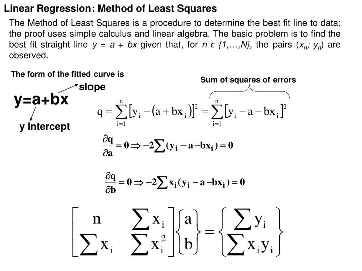
Linear Regression: Method of Least Squares The Method of Least Squares is a procedure to determine the best fit line to data; the proof uses simple calculus and linear algebra. The basic problem is to find the best fit straight line y = a + bx given that, for n ϵ {1,…,N}, the pairs (xn; yn) are observed. The form of the fitted curve is Sum of squares of errors slope y=a+bx y intercept
Data point Fitted curve Example 1: Find a 1st order polynomial y=a+bx for the values given in the Table. clc;clear x=[-5,2,4]; y=[-2,4,3.5]; p=polyfit(x,y,1) x1=-5:0.01:7; yx=polyval(p,x1); plot(x,y,'or',x1,yx,'b') xlabel('x value') ylabel ('y value') a=1.188 b=0.484 y=1.188+0.484x
Data point Fitted curve Example 2: y=200.13 + 8.82x y=a+bx clc;clear x=[0,3,5,8,10]; y=[200,230,240,270,290]; p=polyfit(x,y,1) x1=-1:0.01:12; yx=polyval(p,x1); plot(x,y,'or',x1,yx,'b') xlabel('x value') ylabel ('y value')
Method of Least Squares: Method of Least Squares Intercept Intercept Slope Slope Tensile tests were performed for a composite material having a crack in order to calculate the fracture toughness. Obtain a linear relationship between the breaking load F and crack length a.
Method of Least Squares: with Visual Basic: with Matlab: mls.txt 5 10,0.5 9.25,0.4 9.1,0.35 9.4,0.45 8.5,0.28 clc;clear x=[10,9.25,9.1,9.4,8.5]; y=[0.5,0.4,0.35,0.45,0.28]; p=polyfit(x,y,1) F=8:0.01:12; a=polyval(p,x1); plot(x,y,'or‘,F,a,'b') xlabel('x value') ylabel ('y value')
Method of Least Squares: T (°C) Intercept 212 204 200 Slope Intercept Slope 175 0 5 10 15 t (min.) The change in the interior temperature of an oven with respet to time is given in the Figure. It is desired to model the relationship between the temperature (T) and time (t) by a first order polynomial as T=c1t+c2. Determine the coefficients c1 and c2.
Method of Least Squares: with Matlab: With Visual Basic: mls.txt 4 0,175 5,204 10,200 15,212 clc;clear x=[0,5,10,15]; y=[175,204,200,212]; p=polyfit(x,y,1) t=0:0.01:15; T=polyval(p,x1); plot(x,y,'or',t,T,'b') xlabel('x value') ylabel ('y value')