Download
1 / 27
270 likes | 693 Views
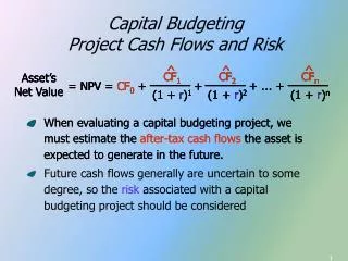
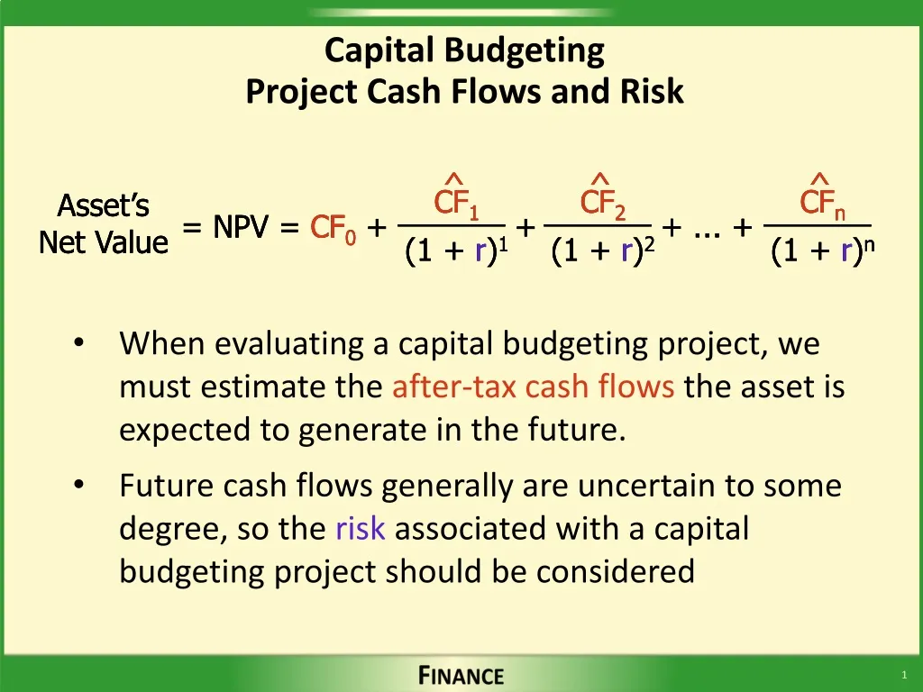
Capital Budgeting Project Cash Flows and Risk. When evaluating a capital budgeting project, we must estimate the after-tax cash flows the asset is expected to generate in the future.

E N D
Capital BudgetingProject Cash Flows and Risk When evaluating a capital budgeting project, we must estimate the after-tax cash flows the asset is expected to generate in the future. Future cash flows generally are uncertain to some degree, so the risk associated with a capital budgeting project should be considered ^ ^ ^ ^ ^ ^ ^ ^ ^ CF1 (1 + r)1 CF1 (1 + r)1 CF1 (1 + r)1 CF2 (1 + r)2 CF2 (1 + r)2 CF2 (1 + r)2 CFn (1 + r)n CFn (1 + r)n CFn (1 + r)n Asset’s Net Value Asset’s Net Value Asset’s Net Value + … + + … + + … + = NPV = CF0+ = NPV = CF0 + = NPV = CF0 + + + +
Capital BudgetingProject Cash Flows and Risk Incremental cash flows = relevant cash flows = marginal cash flows (positive and negative) generated by the asset • Sunk cost • Opportunity cost • Externalities • Shipping and installation • Depreciable basis = Purchase price + (Shipping & Installation) • Inflation
Identifying Incremental (Relevant) Cash Flows Initial investment outlay—includes cash flows that occur only at the beginning of the project’s life. Supplemental operating cash flows—changes in cash flows that are sustained throughout the life of the asset—that is, the cash flow effects are ongoing. Terminal cash flow—the cash flows that occur only at the end of the life of the asset.
Initial Investment Outlay Purchase price Shipping and installation Cost/Benefit of disposing of old asset Taxes Change in net working capital Net working capital = CA – CL Other “up-front” inflows/outflows
Supplemental Operating Cash Flows Δ Cash sales Δ Salaries Δ Costs of raw materials Δ Other cash operating revenues and expenses Δ Taxes Δrevenues or expenses, Δ tax liability Depreciation—non-cash expense that affects the firm’s taxes, which are paid with cash
Terminal Cash Flow Salvage value of new asset Taxes Salvage value of old asset Taxes ΔNet working capital Other “terminal” inflows/outflows associated with both the new asset and the old asset
Capital Budgeting Project Evaluation Expansion projects—marginal cash flows include all cash flows associated with adding a new asset to grow the firm. Replacement analysis—marginal cash flows include changes (+ or -) in the cash flows associated with the new asset that replace the cash flows associated with the old asset that is replaced (maintain existing operations by replacing an old asset).
Expansion Project—Example Increase production by adding a machine • Purchase price$(47,000) • Installation$(3,000) • Life 3 years • Salvage$5,000 • Increase in net WC$(1,500) • Increase in gross profit$21,000 • Marginal tax rate 34% • Depreciation methodMACRS Increase production by adding a machine • Life* • Salvage$5,000 • Increase in net WC* • Marginal tax rate* • Depreciation method* Increase production by adding a machine • Purchase price • Life3 years • Salvage • Increase in gross profit$21,000 • Marginal tax rate* • Depreciation methodMACRS Increase production by adding a machine • Purchase price$(47,000) • Installation$(3,000) • Increase in net WC$(1,500)
Depreciation is used to account for the decrease in the value of a long-term asset during its life. Depreciation is NOT a cash flow. Depreciation affects the taxes a firm pays, because it is a tax-deductible expense. Depreciation
MACRS Depreciation Life Class of Investment Year3-year5-year7-year 133%20%14% 2453225 3151917 471213 5119 669 79 8 4 100%100%100%
Expansion ProjectInitial Investment Outlay Purchase Price$(47,000) Installation( 3,000) Δ Net WC( 1,500) Purchase Price$(47,000) Installation( 3,000) Δ Net WC( 1,500) Initial invest outlay$(51,500) Depreciable basis= $47,000 + $3,000 = $50,000
Expansion ProjectSupplemental Operating Cash Flows Year 1 Year 2 Year 3 D gross profit$21,000$21,000$21,000 Year 1 Year 2 Year 3 D gross profit$21,000$21,000$21,000 Depreciation(16,500) Year 1 Year 2 Year 3 D gross profit$21,000$21,000$21,000 Depreciation(16,500)(22,500) ( 7,500) Depreciation1 = $50,000(0.33) = $16,500 Depreciation1 = $50,000(0.33) = $16,500 Depreciation2 = $50,000(0.45) = $22,500 Depreciation1 = $50,000(0.33) = $16,500 Depreciation2 = $50,000(0.45) = $22,500 Depreciation3 = $50,000(0.15) = $ 7,500
Expansion ProjectSupplemental Operating Cash Flows Year 1 Year 2 Year 3 D gross profit$21,000$21,000$21,000 Depreciation(16,500) Year 1 Year 2 Year 3 D gross profit$21,000$21,000$21,000 Depreciation(16,500)(22,500) Year 1 Year 2 Year 3 D gross profit$21,000$21,000$21,000 Depreciation(16,500)(22,500)( 7,500) Year 1 Year 2 Year 3 D gross profit$21,000$21,000$21,000 Depreciation(16,500)(22,500)( 7,500) D taxable income Year 1 Year 2 Year 3 D gross profit$21,000$21,000$21,000 Depreciation(16,500)(22,500)( 7,500) D taxable income4,500 Year 1 Year 2 Year 3 D gross profit$21,000$21,000$21,000 Depreciation(16,500)(22,500)( 7,500) D taxable income4,500( 1,500) Year 1 Year 2 Year 3 D gross profit$21,000$21,000$21,000 Depreciation(16,500)(22,500)( 7,500) D taxable income4,500( 1,500)13,500 Year 1 Year 2 Year 3 D gross profit$21,000$21,000$21,000 Depreciation(16,500)(22,500)( 7,500) D taxable income4,500( 1,500)13,500 D taxes (34%) Year 1 Year 2 Year 3 D gross profit$21,000$21,000$21,000 Depreciation(16,500)(22,500)( 7,500) D taxable income4,500( 1,500)13,500 D taxes (34%) (1,530) Year 1 Year 2 Year 3 D gross profit$21,000$21,000$21,000 Depreciation(16,500)(22,500)( 7,500) D taxable income4,500( 1,500)13,500 D taxes (34%) (1,530) D net income Year 1 Year 2 Year 3 D gross profit$21,000$21,000$21,000 Depreciation(16,500)(22,500)( 7,500) D taxable income4,500( 1,500)13,500 D taxes (34%) (1,530) D net income2,970 Year 1 Year 2 Year 3 D gross profit$21,000$21,000$21,000 Depreciation(16,500)(22,500)( 7,500) D taxable income4,500( 1,500)13,500 D taxes (34%) (1,530) 510 D net income2,970 Year 1 Year 2 Year 3 D gross profit$21,000$21,000$21,000 Depreciation(16,500)(22,500)( 7,500) D taxable income4,500( 1,500)13,500 D taxes (34%) (1,530) 510 D net income2,970( 990) Year 1 Year 2 Year 3 D gross profit$21,000$21,000$21,000 Depreciation(16,500)(22,500)( 7,500) D taxable income4,500( 1,500)13,500 D taxes (34%) (1,530) 510( 4,590) D net income2,970( 990) Year 1 Year 2 Year 3 D gross profit$21,000$21,000$21,000 Depreciation(16,500)(22,500)( 7,500) D taxable income4,500( 1,500)13,500 D taxes (34%) (1,530) 510( 4,590) D net income2,970( 990)8,910 Year 1 Year 2 Year 3 D gross profit$21,000$21,000$21,000 Depreciation(16,500)(22,500)( 7,500) D taxable income4,500( 1,500)13,500 D taxes (34%) (1,530) 510( 4,590) D net income2,970( 990)8,910 Year 1 Year 2 Year 3 D gross profit$21,000$21,000$21,000 Depreciation(16,500)(22,500)( 7,500) D taxable income4,500( 1,500)13,500 D taxes (34%) (1,530) 510( 4,590) D net income2,970( 990)8,910 Depreciation16,500 Year 1 Year 2 Year 3 D gross profit$21,000$21,000$21,000 Depreciation(16,500)(22,500)( 7,500) D taxable income4,500( 1,500)13,500 D taxes (34%) (1,530) 510( 4,590) D net income2,970( 990)8,910 Depreciation16,500 D operating CF19,470 Year 1 Year 2 Year 3 D gross profit$21,000$21,000$21,000 Depreciation(16,500)(22,500)( 7,500) D taxable income4,500( 1,500)13,500 D taxes (34%) (1,530) 510( 4,590) D net income2,970( 990)8,910 Depreciation16,50022,500 D operating CF19,470 Year 1 Year 2 Year 3 D gross profit$21,000$21,000$21,000 Depreciation(16,500)(22,500)( 7,500) D taxable income4,500( 1,500)13,500 D taxes (34%) (1,530) 510( 4,590) D net income2,970( 990)8,910 Depreciation16,50022,500 D operating CF19,47021,510 Year 1 Year 2 Year 3 D gross profit$21,000$21,000$21,000 Depreciation(16,500)(22,500)( 7,500) D taxable income4,500( 1,500)13,500 D taxes (34%) (1,530) 510( 4,590) D net income2,970( 990)8,910 Depreciation16,50022,5007,500 D operating CF19,47021,510 Year 1 Year 2 Year 3 D gross profit$21,000$21,000$21,000 Depreciation(16,500)(22,500)( 7,500) D taxable income4,500( 1,500)13,500 D taxes (34%) (1,530) 510( 4,590) D net income2,970( 990)8,910 Depreciation16,50022,500 7,500 D operating CF19,47021,51016,410 Year 1 Year 2 Year 3 D gross profit$21,000$21,000$21,000
Expansion ProjectSupplemental Operating Cash Flows Year 1 Year 2 Year 3 D gross profit$21,000$21,000$21,000 Depreciation(16,500)(22,500)( 7,500) D taxable income4,500( 1,500)13,500 D taxes (34%) (1,530) 510( 4,590) D operating CF19,47021,51016,410 DCF1 = (DNOI1 +D Depr1)(1 – T) + TDDepr1 = ($4,500 + $16,500)(1 – 0.34) + 0.34($16,500) = $13,860 + $5,610 = $19,470
Salvage of asset$5,000 Taxes on sale(510) Expansion ProjectTerminal Cash Flow Salvage of asset$5,000 Taxes on sale(510) Δ net working capital1,500 Terminal cash flow 5,990 Salvage of asset$5,000 Taxes on sale(510) Δ net working capital1,500 % of asset depreciated = 33% + 45% + 15% = 93% Book Value = (0.07)$50,000 = $3,500 Gain on sale = Sale price – Book value % of asset depreciated = 33% + 45% + 15% = 93% Book Value = (0.07)$50,000 = $3,500 Gain on sale = $5,000–$3,500 = $1,500 % of asset depreciated = 33% + 45% + 15% = 93% Book Value = (0.07)$50,000 = $3,500 Gain on sale = $5,000–$3,500=$1,500 Tax on gain = 0.34 x $1,500 = $510
0 1 2 3 Expansion ProjectCash Flow Timeline 12% (51,500.00) 19,470 21,510 16,410 5,990 17,383.93 22,400 17,147.64 15,943.88 IRR = 10.9% (1,024.55)
Capital Budgeting Project Risk Project risk should be evaluated to determine whether the appropriate required rate of return is used to compute the project’s NPV (or to compare to its IRR). If a firm is considering a project that is much riskier than the existing assets, then it makes sense that the firm should expect to earn a higher return on the project than on its existing assets, and vice versa.
Capital Budgeting Project Risk Types of risk associated with projects: Stand-alone risk—risk of the asset when it is held in isolation—that is, when it stands alone Corporate, or within-firm, risk—measured by the impact an asset is expected to have on the operations of the firm—that is, how an asset will affect the firm’s total risk if it is purchased and added to existing assets Beta, or market, risk—the portion of an asset’s risk that cannot be eliminated through diversification—that is, how an asset will affect the firm’s market risk, or beta, if it is purchased and added to existing assets.
Sensitivity analysis—determine by how much the final result of a computation, such as NPV, changes when the values (inputs) needed for the computation are changed. Example—replacement decision illustration: Stand-Alone Risk of a Project Operating Expense Required Rate Deviation from Savings per Year of Return (r) Base Case (%) NPV % D NPV % D -10$(421.29)(237%)$519.2769% 0307.680307.680 101,036.6423799.85(68) Operating Expense Required Rate Deviation from Savings per Year of Return (r) Base Case (%) NPV % D NPV % D -10$(421.29)(237%)$519.2769% 0 307.68 0 307.68 0 101,036.6423799.85(68) Operating Expense Required Rate Deviation from Savings per Year of Return (r) Base Case (%) NPV % D NPV % D -10$(421.29) (237%)$519.2769% 0307.680307.680 101,036.64 237 99.85(68) Operating Expense Required Rate Deviation from Savings per Year of Return (r) Base Case (%) NPV % D NPV % D -10$(421.29)(237%)$519.2769% 0307.680307.680 101,036.6423799.85(68)
Scenario analysis—compute outcomes using various circumstances, or scenarios. Stand-Alone Risk of a Project Scenario Savings NPVProbability Best case$10,000$3,9530.2 Most likely case8,0003080.7 Worst case6,000(3,337)0.1 Scenario Savings NPVProbabilityNPV x Pr Best case$10,000$3,9530.2$790.60 Most likely case8,0003080.7215.60 Worst case6,000(3,337)0.1(333.70) (333.70) Expected NPV = 672.50 (333.70) Expected NPV = 672.50 sNPV = 1,962.89 (333.70) Expected NPV = 672.50 sNPV = 1,962.89 CVNPV =2.92
Monte Carlo simulation—try to simulate the real world by identifying all the possible outcomes for all the situations, or variables, that are associated with a capital budgeting project. Stand-Alone Risk of a Project
Determine how a capital budgeting project is related to the existing assets of the firm. If the firm wants to diversify its risk, it will try to invest in projects that are negatively related (or have little relationship) to the existing assets. If a firm can reduce its overall risk, then it generally becomes more stable and its required rate of return decreases. Corporate (Within-Firm) Risk
Theoretically any asset has a beta,, or some way to measure its systematic risk If we can determine the beta of an asset, then we can use the capital asset pricing model, CAPM, to compute its required rate of return as follows: rproj = rRF + (rM - rRF)proj Measuring beta risk for a project—it is difficult to determine the beta for a project. pure play method Beta (Market) Risk
Beta (Market) Risk • Capital Budgeting Project Characteristics: Cost= $100,000 βproject= 1.5 rRF= 3.0% rM= 9.0% rproject= 3.0% + (9.0% - 3.0%)1.5 = 12.0% • Firm’s Characteristics Before Purchasing the Project: Total assets = $400,000 β Firm-current= 1.0 • Firm’s Beta Coefficient After Purchasing the Project: Total assets = $400,000 + $100,000 = $500,000
The firm generally uses its average required rate of return to evaluate projects with average risk. The average required rate of return is adjusted to evaluate projects with above-average or below-average risks. Capital Budgeting—Risk Analysis Project Required Risk Category Rate of Return Above-average 16% Average 12 Below-average 10 • If risk is not considered, high-risk projects might be accepted when they should be rejected and low-risk projects might be rejected when they should be accepted.
Multinational Capital Budgeting Capital budgeting projects of multinational firms should be evaluated using the same techniques. Repatriation of cash might restrict cash flows. Projects associated with foreign operations generally are considered riskier than domestic projects because: Movements in exchange rates—that is, exchange rate risk. Political risk—risk that foreign governments will takeover or severely restrict operations of foreign subsidiaries (risk of expropriation)
Chapter 10 Questions What are the relevant cash flows associated with a capital budgeting project? What is depreciation and how does it affect a project’s relevant cash flows? How is risk incorporated in capital budgeting analysis? How do capital budgeting analyses/decisions differ for multinational firms?