Graphite monolayers

1. Graphite monolayers Edward McCann Lancaster University, UK with S. Bailey, K. Kechedzhi, V.I. Fal’ko, H. Suzuura, T. Ando, B.L. Altshuler

2. Graphite Three dimensional layered material with hexagonal 2D layers [shown here with Bernal (AB) stacking]

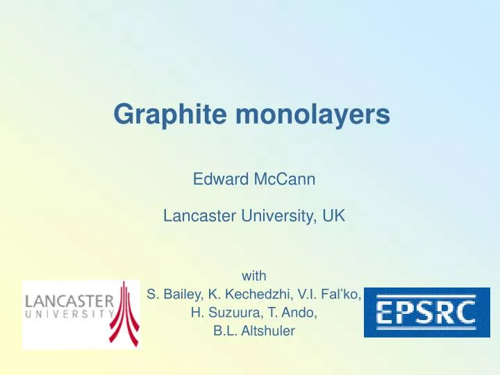
3. Graphite Monolayer Two dimensional material; zero gap semiconductor; Dirac spectrum of electrons Three dimensional layered material with hexagonal 2D layers [shown here with Bernal (AB) stacking]

4. Graphite Monolayer Two dimensional material; zero gap semiconductor; Dirac spectrum of electrons Bilayer Three dimensional layered material with hexagonal 2D layers [shown here with Bernal (AB) stacking] Bilayer as a 2D material Low energy Hamiltonian= ?

5. Graphite Bilayer Monolayer Two dimensional material; zero gap semiconductor; Dirac spectrum of electrons Two dimensional material; Low energy Hamiltonian? Fabricated two years ago by Manchester group, Novoselov et al, Science 306, 666 (2004). Three dimensional layered material with hexagonal 2D layers [shown here with Bernal (AB) stacking] Further reports of quantum Hall effect measurements; Manchester group:Novoselov et al, Nature 438, 197 (2005) Columbia group: Zhang et al, Nature 438, 201 (2005).

6. Graphite Bilayer Monolayer Two dimensional material; zero gap semiconductor; Dirac spectrum of electrons Two dimensional material; Low energy Hamiltonian? Lecture Overview 1) Tight binding model of monolayer graphene 2) Expansion near the K points: chiral quasiparticles and Berry phase 3) Bilayer graphene 4) Quantum Hall effect Three dimensional layered material with hexagonal 2D layers [shown here with Bernal (AB) stacking]

7. 1 Tight binding model of monolayer graphene “Physical Properties of Carbon Nanotubes” R Saito, G Dresselhaus and MS Dresselhaus; Imperial College Press, 1998

8. 1 Tight binding model of monolayer graphene1.1 sp2 hybridisation • Carbon has 6 electrons • 2 are core electrons • 4 are valence electrons – one 2s and three 2p orbitals

9. 1 Tight binding model of monolayer graphene1.1 sp2 hybridisation • Carbon has 6 electrons • 2 are core electrons • 4 are valence electrons – one 2s and three 2p orbitals • sp2 hybridisation • single 2s and two 2p orbitals hybridise forming three “s bonds” in the x-y plane

10. 1 Tight binding model of monolayer graphene1.1 sp2 hybridisation • Carbon has 6 electrons • 2 are core electrons • 4 are valence electrons – one 2s and three 2p orbitals • sp2 hybridisation • remaining 2pz orbital [“p” orbital] exists perpendicular to the x-y plane only p orbital relevant for energies of interest for transport measurements – so keep only this one orbital per site in the tight binding model

11. 1 Tight binding model of monolayer graphene1.2 lattice of graphene 2 different ways of orienting bonds means there are 2 different types of atomic sites [but chemically the same]

12. 1 Tight binding model of monolayer graphene1.2 lattice of graphene 2 different atomic sites – 2 triangular sub-lattices

13. 1 Tight binding model of monolayer graphene1.3 reciprocal lattice triangular reciprocal lattice – hexagonal Brillouin zone

14. 1 Tight binding model of monolayer graphene1.4 Bloch functions We take into account one p orbital per site, so there are two orbitals per unit cell. Bloch functions sum over all type B atomic sites in N unit cells atomic wavefunction

15. 1 Tight binding model of monolayer graphene1.4 Bloch functions We take into account one p orbital per site, so there are two orbitals per unit cell. Bloch functions : label with j = 1 [A sites] or 2 [B sites] sum over all type j atomic sites in N unit cells atomic wavefunction

16. 1 Tight binding model of monolayer graphene1.5 Secular equation Eigenfunction Yj(for j = 1 or 2) is written as a linear combination of Bloch functions: Eigenvalue Ej(for j = 1 or 2) is written as :

17. 1 Tight binding model of monolayer graphene1.5 Secular equation Eigenfunction Yj(for j = 1 or 2) is written as a linear combination of Bloch functions: Eigenvalue Ej(for j = 1 or 2) is written as : substitute expression in terms of Bloch functions defining transfer integral matrix elements and overlap integral matrix elements

18. 1 Tight binding model of monolayer graphene1.5 Secular equation

19. 1 Tight binding model of monolayer graphene1.5 Secular equation If the and are known, we can find the energy by minimising with respect to :

20. 1 Tight binding model of monolayer graphene1.5 Secular equation

21. 1 Tight binding model of monolayer graphene1.5 Secular equation Explicitly write out sums:

22. 1 Tight binding model of monolayer graphene1.5 Secular equation Explicitly write out sums: Write as a matrix equation:

23. 1 Tight binding model of monolayer graphene1.5 Secular equation Explicitly write out sums: Write as a matrix equation: Secular equation gives the eigenvalues:

24. 1 Tight binding model of monolayer graphene1.6 Calculation of transfer and overlap integrals

25. 1 Tight binding model of monolayer graphene1.6 Calculation of transfer and overlap integrals Diagonal matrix element Same site only:

26. 1 Tight binding model of monolayer graphene1.6 Calculation of transfer and overlap integrals Diagonal matrix element Same site only: A and B sites are chemically identical:

27. 1 Tight binding model of monolayer graphene1.6 Calculation of transfer and overlap integrals Diagonal matrix element Same site only: A and B sites are chemically identical:

28. 1 Tight binding model of monolayer graphene1.6 Calculation of transfer and overlap integrals Off-diagonal matrix element

29. 1 Tight binding model of monolayer graphene1.6 Calculation of transfer and overlap integrals Off-diagonal matrix element Every A site has 3 B nearest neighbours:

30. 1 Tight binding model of monolayer graphene1.6 Calculation of transfer and overlap integrals Off-diagonal matrix element Every A site has 3 B nearest neighbours:

31. 1 Tight binding model of monolayer graphene1.6 Calculation of transfer and overlap integrals Off-diagonal matrix element Every A site has 3 B nearest neighbours: Parameterise nearest neighbour transfer integral:

32. 1 Tight binding model of monolayer graphene1.6 Calculation of transfer and overlap integrals Off-diagonal matrix element Every A site has 3 B nearest neighbours: Parameterise nearest neighbour transfer integral:

33. 1 Tight binding model of monolayer graphene1.6 Calculation of transfer and overlap integrals Off-diagonal matrix element

34. 1 Tight binding model of monolayer graphene1.7 Calculation of energy

35. 1 Tight binding model of monolayer graphene1.7 Calculation of energy Secular equation gives the eigenvalues:

36. 1 Tight binding model of monolayer graphene1.7 Calculation of energy Secular equation gives the eigenvalues:

37. 1 Tight binding model of monolayer graphene1.7 Calculation of energy Typical parameter values [quoted in Saito et al]:

38. 2 Expansion near the K points2.1 Exactly at the K point At the corners of the Brillouin zone (K points), electron states on the A and B sub-lattices decouple and have exactly the same energy K points also referred to as “valleys”

39. 2 Expansion near the K points2.1 Exactly at the K point 6 corners of the Brillouin zone (K points), but only two are non-equivalent We consider two K points with the following wave vectors: K K’ b1 b2 K K’

40. 2 Expansion near the K points2.2 Linear expansion Consider two non-equivalent K points: p and small momentum near them:

41. 2 Expansion near the K points2.2 Linear expansion Consider two non-equivalent K points: p and small momentum near them: Linear expansion in small momentum:

42. 2 Expansion near the K points2.2 Linear expansion New notation for components on A and B sites

43. 2 Expansion near the K points2.3 Dirac-like equation For one K point (e.g. x=+1) we have a 2 component wave function, with the following effective Hamiltonian: Bloch function amplitudes on the AB sites (‘pseudospin’) mimic spin components of a relativistic Dirac fermion.

44. 2 Expansion near the K points2.3 Dirac-like equation To take into account both K points (x=+1 and x=-1) we can use a 4 component wave function, with the following effective Hamiltonian:

45. Helical electrons pseudospin direction is linked to an axis determined by electronic momentum. for conduction band electrons, valence band (‘holes’) 2 Expansion near the K points2.3 Dirac-like equation

46. 2 Expansion near the K points2.4 Absence of backscattering

47. 2 Expansion near the K points2.4 Absence of backscattering angular scattering probability: j = 0 under pseudospin conservation, helicity suppresses backscattering in a monolayer

48. 2 Expansion near the K points2.5 Berry’s phase p

49. Monolayer graphene massless Dirac fermions with Berry’s phase p

50. 3. Bilayer graphene [Bernal (AB) stacking]