Download
1 / 19
190 likes | 364 Views
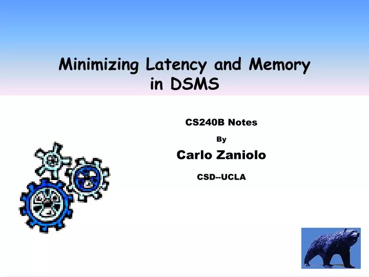
Minimizing Latency and Memory in DSMS. CS240B Notes By Carlo Zaniolo CSD--UCLA. Query Optimization in DSMS Opportunities and Challenges. ∑1. Sink. O 2. Source. σ. ∑ 2. Sink. Source. O 1. Sink. O 3. . ∑ 1. Sink. Source1. U. Source2. σ. ∑ 2. Sink.

E N D
Minimizing Latency and Memory in DSMS CS240B Notes By Carlo Zaniolo CSD--UCLA
Query Optimization in DSMSOpportunities and Challenges ∑1 Sink O2 Source σ ∑2 Sink Source O1 Sink O3 ∑1 Sink Source1 U Source2 σ ∑2 Sink • Simple DBMS-like opportunities: e.g. pushing selection. • Sharing of operators and buffers can be important. • No Major saving in execution time from reordering, indexes and operator implementation. Except for these cases: • Total execution time is determine by the query graphs and the buffer contents.
Optimization Objectives • Rate-based optimization [VN02]: Overall objective is to maximize the tuple output rate for a query • Minimize Memory Consumption: with large buffer memory could become scarce • Minimize response time (latency): • Time from source to sink • Maximize user satisfaction
Rate Based Optimization • Rate-based optimization [VN02]: • Take into account the rates of the streams in the query evaluation tree during optimization • Rates can be known and/or estimated • Overall objective is to maximize the tuple output rate for a query • Instead of seeking the least cost plan, seek the plan with the highest tuple output rate. • maximizing output rate normally leads to optimum response-time. But no actual proof of that. • As opposed to Chain that guarantees optimality for memory [Babcock 2003]
Progress charts • Each step represents an operator • The ith operator takes (ti – ti-1) units of time to process a tuple of size si-1 • Result is a tuple of size si • We can define selectivity as the drop in tuple size from operator i to operator i+1. O1 Source O2 O3 O1 O2
Chain Scheduling Algorithm Source O1 O2 O3 Sink Original query graph is partitioned into sub-graphs that are prioritized eagerly O1 O1 Lower Memory Memory O2 O2 envelope O3 O3 Time
State of the Art • Chain Limitations: • Latency minimization not supported—only memory • Generalization to general graphs leaves much to be desired • Assumes every tuple behaves in the same way • Optimality achieved only under this assumption---what about if tuples behave differently?
Query Graph: Arbitrary DAGs Source1 U Sink Source2 σ Sink O2 Source σ ∑1 ∑2 Sink Source O1 Sink O3 ∑1 Sink Source1 U Source2 σ ∑2 Sink
Chain for Latency Minimization? • Chain Contributions: • Use the efficient chart partitioning algorithm to break up each component into subgraphs, where • resulting subgraphs are scheduled greedly (steepest slope first). • How can that be used to minimize latency on arbitrary graphs? (assuming that the idle-waiting problem has been solved--or does not occur because of massive and balanced arrivals).
Example, one operator: Latency: the Output Completion Chart Total Output Remaining Output 3 3 2 Remaining Output 2 1 N 1 Time Time Source O1 Sink tuple1 tuple2 tuple3 tuple1 tuple2 tuple3 S Time • Suppose we have 3 input tuples at operator O1 • Horizontal axis is time, vertical axis is # remaining output to be produced • Many waiting tuples curve smoothes into the dotted slope • The slope is average tuple processing rate
Latency Minimization Remaining Output O1 O2 O3 O4 Time A: Source O1 Sink B: Source O2 Sink Remaining Output: A first • Example for latency optimization: multiple independent operators • Total area under the curve represents total latency over time • Minimizing total area under the curve—same as lower envelope • Order operators by non-increasing slopes B first B SB A SA A B SB Time SA Time
Latency Optimization on Tuple-Sharing Fork O1+O2 2N 2N O1+O2 O1+O2+O3 O1+O2+O3 N O3 N O3 Time Time N(1 + 2+3 ) N x 3 N(1+2) Sink Sink O2 O2 Source Source O1 O1 Sink Sink O3 O3 Tuples shared by multiple branches: scheduling choices at forks: • Finish all tuples on the fastest branch first (break the fork) • Achieve fastest rate over the first branch • Take each input through all branches (no break) • FIFO , achieves the average rate of all branches Partition at Fork No Partition atFork
Latency Optimization on Nested Fork E D Remaining Output G+H+P C+A+B O A Sink C B Sink D Sink Source E H Sink P Sink G O Sink • Recursively apply the partitioning algorithm from bottom-up • Starting from forks closest to sink buffers • Similar algorithms can be used for memory minimization • Slopes are memory-reduction rates • Require branch-segmentation, more complicated
Optimal Algorithm-Latency Minimization Source A Sink Source B Sink Source C Sink • We have so far assumed which buffer to process next by the average costs of the tuples in each buffer. Thus for the simple case above the complete schedule is a permutation of A, B, and C. • Scheduling based on individual tuple cost: make a scheduling decision for each tuple and the basis of its individual cost. • Scheduling is still constrained by tuple-arrival order—thus at each step, we chose between the heads of each buffer. • A greedy approach that selects the least expensive head is not optimal!
Optimal Algorithm:when cost of each tuple is known Source A Sink Source B Sink Source C Sink • For each buffer chart the costs of the tuples in the buffer: Partion each chart into groups of tuples • Schedule group of tuples eagerly, i.e. by decreasing slope • Optimality as minimization of resulting:area = cost × time.
Example: Optimal Algorithm Source A Sink Source B Sink A5,A4,A3,A2,A1 B3,B2,B1 \ / \ / A1 A2 a B1 B2 SA1 A3 SB1 A4 B3 A5 Time SB2 Time SA2 • * Naïve Greedy would take B1 before A1 • ** Optimal Order: SA1=A1,A2,A3,A4. Then SB1=B1,B2, then SB2=B3, finally SA2=A5.
Experiments – Practical vs. Optimal Latency Minimization Over many tuples, the practical component-based algorithm for latency minimization closely resemble the performance of the (unrealistic) optimal algorithm.
Results • Unified scheduling algorithms for both latency and memory optimization • The proposed algorithms are based on the chart-partitioning method first used by Chain for memory minimization • Also a better memory minimization for tuple-sharing forks. • Derived optimal algorithms under the assumption that the processing costs of individual tuples is known. • Experimental evaluation shows that optimization based on the average costs of tuples in buffer (instead of their individual costs ) produces nearly optimal results.
References S. Viglas, J. F. Naughton: Rate-based query optimization for streaming information sources. SIGMOD Conference 2002: 37-48 [VN02] B. Babcock, S. Babu, M. Datar, R. Motwani: Chain: Operator Scheduling for Memory Minimization in Data Stream Systems. SIGMOD Conference 2003: 253-264 This is the chain paper referred to as [BBDM03] or [Babcock et al.] Yijian Bai and Carlo Zaniolo: Minimizing Latency and Memory in DSMS: a Unified Approach to Quasi-Optimal Scheduling. The Second International Workshop on Scalable Stream Processing Systems, March 29, 2008, Nantes, France.