Download
1 / 81
810 likes | 817 Views
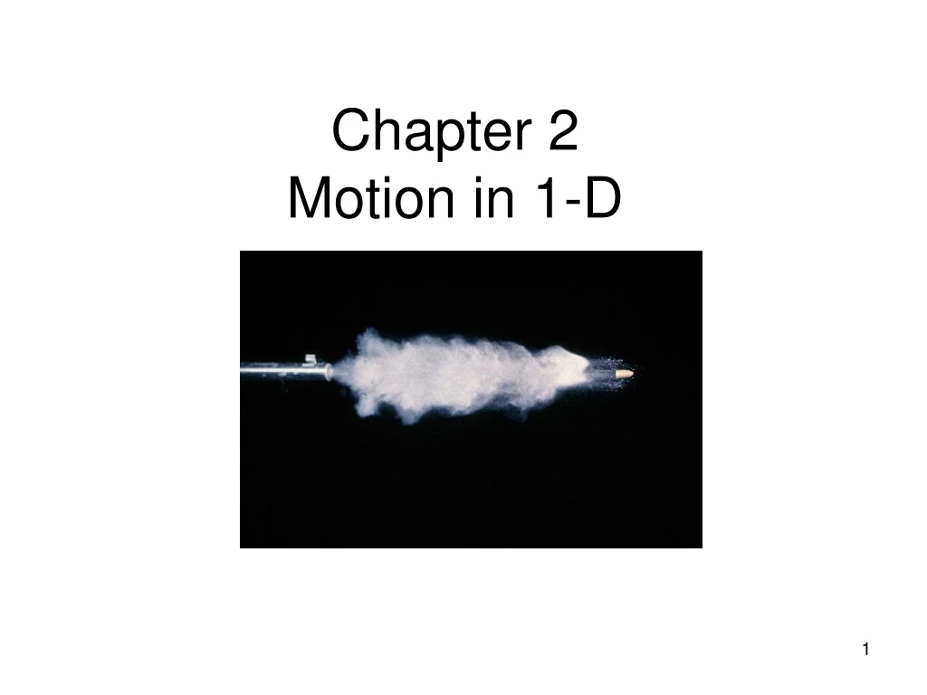
Chapter 2 Motion in 1-D. Kinematics. Kinematics is the branch of classical mechanics that describes the motion of objects without consideration of the causes leading to the motion. Only 1-D motion (along a line) be discussed in this chapter. Approximation.

E N D
Kinematics • Kinematics is the branch of classical mechanics that describes the motion of objects without consideration of the causes leading to the motion. • Only 1-D motion (along a line) be discussed in this chapter.
Approximation • To ease discussion, an object with extended size will be modeled as a point
How to describe the motion of a particle in 1-D • Choose a reference coordinate system (an origin and directions) • Assign the position of the particle, x = x(t) • In the example below, direction pointing to the right is +ve, to the left is –ve. • Knowing x at anytime t means we know where the particle is located Origin O x(t) > 0 x(t) < 0
Example of assigning position is located at the position x = 15. It means the location of is at 10 unit to the right of the reference point O (called the origin) at time t. is located at the position x = -10. It means the location of is at 10 unit to the left of the reference point O (called the origin) at time t. Origin O x(t) = +15 x(t) = -10
Example of assigning position • If x(t) > 0 it means the location is to the right of the origin • If x(t) < 0 it means the location is to the left of the origin • The location depends on: (1) |x(t)| (ii) the sign of x(t) Origin O x(t) = +15 x(t) = -10
Position of a particle is usually a function of time, x(t). x(t) provides the quantitative knowledge of how the particle moves. The position-time graph is very useful to graphically describe the motion of the particle as a function of time. Position-Time Graph Active figure 2.1
Defined as the change in position during some time interval Represented as x x = xf- xi SI units are meters (m) x can be positive or negative Displament B from A = position at B – position at A = (+ 52 m) – (30 m) = + 22 m. The negative sign infers the displacement is in the positive direction Displacement
Displacement is defined by two end points • It takes two points to define a displacement. • Say a particle moves from point A to B after some time interval. The displacement is defined as the vector A ends at tB B begins at tA
Displacement of E from C = position at E – position at C = (-37 m) – (+38m) = -75 m The negative sign infers the displacement is in the negative direction Displacement is a vectorial quantity (because it has a sense of direction) It is a “path-independent” quantity, i.e. it depends only on the initial and final positions but not on the path or the specific way the change of position takes place. Example of displacement
Distance traversed in 1-D • Say a particle moves from point A (at time tA) and finally stops at point B (at time tB) • Distance traversed (DT) by the particle when travelling from A to B is the total distance experienced by the particle between the time interval tAtB • Note that there are many ways the particle can move from A to B within the time interval tAtB A ends at tB B begins at tA
Example of distance traversed in 1-D • TD via path I and path II are different, despite the displacement for both path are the same, namely • For path I, DT is • For path II, DT is • DT between two points is a path-dependent quantity • It is an accumulative quantity and must be positive. Path II A C B Path I
Quiz • Is DT a scalar or a vector? • Can DT = |displacement|? • When? • Is it possible that displacement =0 yet DT ≠ 0. If yes, when? • Given the function x(t), how would you obtain DT as a function of time? • Would DT ever decrease as time grows? Why?
Mean velocity • The rate at which displacement happens within a temporal interval • Geometrically it is represented by the slope of the straight line connecting the end positions in the graph of position vs. time • SI Unit: m/s • Is mean velocity a vectorial quantity or a scalar quantity?
Mean speed • Definition: distance traversed / time interval • Speed is a scalar quantity • Same unit as velocity • Generally, mean speed in an finite temporal interval is not equal to the magnitude of the mean velocity.
Can mean speed be negative valued? Generally, is mean speed = |mean velocity| between two points? In a swimming contests, does the swimmers concern about average velocity or average speed? Quiz
Quiz • A Porche dashes off from rest from a starting point, and returned 10s later after making a U-turn 70 m away. • Sketch the x-t curve for the Porche, label it appropriately. • What is the average velocity of the Porche in the 10 s temporal interval? • How would you estimate the average speed in the 10 s temporal interval based on the x(t) curve?
Instantaneous velocity • Definition: The limit of mean velocity when Dt0 • It could be positive, zero, or negative. • It tells us what is the state of motion of the object changes from moment to moment.
Obtaining instantaneous velocity from a x(t) curve • Instantaneous velocity at any moment is given by the slope of the tangent to the point on the curve x(t) at t. • Example: the instantaneous velocity at A can be obtained as the limit of the slope AB as BA (corresponds to letting Dt0) Active figure 2.3
Instantaneous speed • Defined as the magnitude of instantanous velocity. • In general, mean speed ≠ |mean velocity| in a finite time interval Dt. • However, in the limit Dt 0, mean speed = |mean velocity| because mean speed becomes instantaneous speed, and mean velocity become instantaneous velocity.
Example • A particle moves along the x-axis according to x(t) = -4t + 2t2 • x in m, t in seconds • (A) Determine displacement of the particle in the time interval t = 0 t = 1s and t = 1s t = 3s.
Solution (A) • x(t) = -4t + 2t2 • xAB = xB - xA = -2 m • xBD = xD - xB =+8 m +x B A D
(B) Calculate the mean velocities for the two intervals Solution: • In interval t = 0 t = 1s, • t = tf – ti = (1 – 0)s = 1 s • Mean velocity = • In the time inverval t = 1s t = 3s, t = 2s
(C) Calculate the instantaneous velocity of the particle at t = 2.5 s Solution: • Measure the slop of the tangent to the curve at C: • Alternatively, vC can also be evaluated by taking the derivative dx/dt at t=2.5 s
Mean acceleration • Definition: the change in velocity v divided by the time interval Dt in which the change takes place. • Dimension = L/T2 • SI unit = m/s²
Instantaneous acceleration • Definition: the limit of mean acceleration as t0 • The slope of the graph of velocity vs. time at the point B = instantaneous acceleration at B
Constant acceleration • Object with constant velocity: the acceleration is zero
a parallel with v • Object’s speed increases as function of time if acceleration (non-zero) and velocity is in the same direction. • The above show the case of a constant acceleration in the same direction as the velocity.
a anti-parallel with v • Object’s speed decreases as function of time if acceleration (non-zero) and velocity is in the opposite direction. • The above shows the case of a constant acceleration in the opposite direction as the velocity. • This is sometime called ‘deceleration’ Active figure 2.9
Kinematic graphs • The right exemplify graphically the relations among position, instantaneous velocity and acceleration (x, v, a) as a function of t. • velocity = slope of the x-t curve • Acceleration = slope of the v-t curve
Example • Given v = (40 - 5t2) m/s, t in seconds. • We calculated the average acceleration within any time interval • vi = (40 – 5t2)m/s • After some time interval t, • vf = 40 – 5(t + t)2 m/s • Hence the change in velocity in Dt is • v = vf – vi = [-10t t – 5(t)2] m/s • By definition:
The instantaneous acceleration at t = 2 s, a (t = 2) = -10 (2.0) m/s2 = -20 m/s2 Example (cont.)
1-D Kinematics at constant acceleration • Consider a particle is moving along in the x-direction with the conditions that • (i) the acceleration ax is constant, • (ii) initial position xi and velocity vxi • The position xf and velocity vxf at any time t later are determined by a set of kinematic equation.
Notes • Unless mentioned explicitly, the term ‘velocity’ will mean ‘instantaneous velocity’, ‘speed’ will mean ‘instantaneous speed’
1D Kinematic equations at constant acceleration • The equations are used to solve the motion problem of a particle in constant acceleration.
The displacement - time curve at constant acceleration • The slope of the curve is the velocity • A curved line indicates the velocity is changing, therefore, a non-zero acceleration • If it is a straight line, no velocity change happen, hence acceleration = 0.
The velocity – time curve at constant acceleration • The slope gives the acceleration • The straight line indicates a constant acceleration • If the line is flat, (slope zero), it means zero acceleration. • Area under the v-t curve in the time interval Dt = t2-t1 is the distance traversed in this time interval.
The acceleration – time curve at constant acceleration • The zero slope indicates a constant acceleration Active figure 2.10 Active figure 2.11
Quiz • How do I calculate the kinematic problem of a particle moving with non-constant acceleration?
Example: Saga accelerates • In a hypothetical scenario, a proton Saga accelerates from rest to a speed of 42.0 m/s in 8.0 second. Assuming the acceleration is constant, determine the acceleration.
Solution • From the kinematic equation which is in fact the definition of acceleration • Note: Actually, realistically, the acceleration of the Proton Saga changes with time and is not a constant as assumed.
Find the distance traversed by the Proton in the first 8 second • Choose the origin O to be coincident with the point xi = 0 in the kinematic equation. • Initial condition: at, t = 0, x = xi = 0, x=vxi = 0 • Alternatively written as x(t=0) = xi=0, vx(t=0) = vxi=0 • Here, initial position, initial velocity and acceleration are known, and we want to know the final position xf(t) in terms of these. • Slot in the initial condition, xf = 0 + 0t+ (5.25 m/s2) (8s)2 = 168 m
Find the velocity of the Proton after 8.0 s • We wish to find vxf given the knowledge of the constant acceleration and initial conditions x(t=0) = xi=0, vx(t=0) = vxi=0 • The final velocity as a function of time is • Hence vxf = 0 + (5.25 m/s2) (8.0 s)2 = … m
Say you are traveling at constant speed 50 m/s in a car passing by a sign board, behind which a policeman is hiding. After 1 second you pass by, the policeman accelerate at a constant acceleration 3.00 m/s2 to go after you. How long it takes for the policeman to catch up with you? The problem is best solved graphically. Speed trapping
Solution • Use the fact that distance traversed = area under the v-t curve v Your constant velocity vu= 50m/s Function of the velocity of the policeman as a function of time in general takes the form of v = u + at t O t’, time when the policeman catch up with your car t=1s
Solution • Determine the linear equation for the policeman’s velocity, given the a = 3.00 m/s2 and initial condition v (t=1) = 0. • v = u + a t 0 = u + 3(1) u = -3 • The function of velocity of the policeman is v = -3 m/s + (3m/s2)t v Your constant velocity vu= 50m/s v = -3 m/s + (3m/s2)t t O t’, time when the policeman catch up with your car t=1s
Area of the square = your distance traversed between t = 0 t = t’ Area of triangle = distance traversed by the policeman between t = 1s and t = t’ Solution • Determine the linear equation for the policeman’s velocity, given the a = 3.00 m/s2 and initial condition v (t=1) = 0. • v = u + a t 0 = u + 3(1) u = -3 • The function of velocity of the policeman is v = -3 m/s + (3m/s2)t v Your constant velocity vu= 50m/s v = -3 m/s + (3m/s2)t t O t’, time when the policeman catch up with your car t=1s
Area of the square = your distance traversed between t = 0 t = t’ Area of triangle = distance traversed by the policeman between t = 1s and t = t’ Solution • Equate area of the square = area of the triangle: • (50 m/s) t’ = (t ’ – 1s)[-3 m/s + 3(m/s2)t’]/2 • (t’)2 - 32t’ + 1 = 0 • t’ = 32.0 s v Your constant velocity vu= 50m/s v = -3 m/s + (3m/s2)t t O t’, time when the policeman catch up with your car t=1s
Definition: a object that moves freely solely under the influence of gravity, where other external forces such as air friction Free fall motion is a constantly accelerated motion in one dimension In free fall, the acceleration does not depend on the mass nor the initial conditions of the object (such as initial position or initial velocity) Freely falling object